Now that we have talked about the differences between FanDuel vs DraftKings scoring, we need to touch on how this will actually impact our strategy. Since we will be creating a mathematical model eventually, this can be easily adjusted. We will be able to account for these differences in our projected points automatically.
However, it will be helpful to take a moment to think about what we expect to change before jumping into it. I generally recommend this for any math problem or application of math concepts. It is very helpful to think about what result you expect ahead of time so you will have some idea at the end if something went horribly wrong and your answer is not even reasonable.
Unfortunately, this happens sometimes. But if you recognize it, you have the chance to fix the error instead of submitting several paid DFS lineups based on a flawed system. This would not end well (as you might expect), so it’s best to avoid it.
For reference, here is a breakdown of everything that gets points for an MLB contest on both sites.
Differences For Hitters Between FanDuel and DraftKings
Both sites give you +3 points if your player hits a single. However, on FanDuel all extra base hits are worth more than they are on DraftKings. Also, getting a Walk or Hit by Pitch is worth the same as a single in FanDuel, while DraftKings only gives +2 points for those. DraftKings also values an RBI and a Run at +2 points, while they are worth +3.5 and +3.2 points respectively on FanDuel.
This means that relatively speaking, a player getting extra base hits and creating runs for their team through RBI, Runs, Stolen Bases, and getting on base without hits is more valuable on FanDuel than it is on DraftKings. Instead, a player with a lot of singles would have relatively higher value on DraftKings. So, we might expect stats like OBP (On Base Percentage) or SLG (Slugging Percentage) to be more correlated to fantasy points on FanDuel, and a stat like AVE (Batting Average) to be more correlated to fantasy points on DraftKings.
Differences For Pitchers Between FanDuel and DraftKings
The main difference between the two scoring systems here, is what pitchers actually receive points for. In DraftKings, things like walks and hits allowed matter. They directly take fantasy points away from the pitcher. This is not the case in FanDuel. FanDuel really only looks at ER (Earned Runs Allowed), Strike Outs, and IP (Innings Pitched).
Because of these differences, we might expect pitchers with a low ERA (Earned Run Average), who pitch more innings, or who throw a lot of Strike Outs to be more valuable in FanDuel. Similarly, we might expect players with a low WHIP (Walks and Hits allowed per Inning Pitched) to be more valuable in DraftKings.
Final Thoughts on Scoring Differences
I do not want to go into too much detail on why these differences matter yet. I just wanted to get you thinking about them a bit now so you can keep that in mind as we build up to more detail on the topic.
Next, we are going to discuss the different game modes offered by FanDuel and DraftKings. Similar to the scoring differences, we will dive into how the differences in rules between game modes will impact our lineup creating strategy. If you want to be notified via email when these posts go up, just put your information in the form below and I’ll let you know as I post them.
If you want to play along and enter some FanDuel lineups of your own as we conduct this investigation, you can use my FanDuel referral link here to get a deposit bonus. You should just need to deposit at least $15 within 30 days of signing up, and you’ll get a $15 bonus added to your account if you use that link.
Some links in this article may be affiliate links or referral links, meaning I would get a small commission for your purchase at no additional cost to you.
We should start by discussing the difference between the scoring systems used for FanDuel vs DraftKings. Their scoring for MLB (baseball) contests are similar, but not exactly the same. We will need to keep these differences in mind as we build our FanDuel lineup optimizer. And you will need to keep them in mind if you plan to adapt the methods I discuss to use them in DraftKings.
FanDuel vs DraftKings Scoring for MLB
FanDuel Scoring for MLB
As of the time of this writing, the table below shows the fantasy points received for each stat a player records.
* Fractional scoring per out. Notes: Quality Start is awarded to a starting pitcher who completes at least six innings and permits no more than three earned runs.
DraftKings Scoring for MLB
Hitters
Pitchers
1B (Single) = +3 points
W (Win) = +4 points
2B (Double) = +5 points
ER (Earned Run) = -2 points
3B (Triple) = +8 points
SO (Strikeout) = +2 points
HR (Home Run) = +10 points
IP (Innings Pitched) = +2.25 points (+0.75 Pts / Out)
Notes: Hitting statistics for Pitchers will not be counted, and Pitching statistics for Hitters will not be counted.
Which will we use?
For the posts that will follow, we will be using FanDuel scoring. However, feel free to consider how the methods described in these posts can be adapted to the DraftKings scoring. If you are a DraftKings player, or prefer that scoring system, I will do my best to present the topics we use in a way that you can use them yourself.
It is my goal for this series of posts that you will be able to take the methods I use and write about to do your own experiments. This means it should be simple for you to change the points received for each stat category and create your own system for DraftKings or any other Daily Fantasy Sports site.
If you want to play along and enter some FanDuel lineups of your own as we conduct this investigation, you can use my FanDuel referral link here to get a deposit bonus. You should just need to deposit at least $15 within 30 days of signing up, and you’ll get a $15 bonus added to your account if you use that link.
Some links in this article may be affiliate links or referral links, meaning I would get a small commission for your purchase at no additional cost to you.
As a math tutor, people have always asked me: how is calculus used in real life? There are many examples of calculus in the real world, and statistics in the real world too. These applications appear in all kinds of industries, and overlapping with other sciences. However, there is one field that has always interested me most: sports.
I have always been fascinated by people using statistics and math to predict the outcome of sporting events. Or even to evaluate the performance of players, their impact on the outcome of the game, and their value to their team. However, I do not work in the sports world. I do not need to inform decisions about what players Billy Bean wanted to sign. I have no input on how big of a contract the Atlanta Braves should offer their 1st baseman with a career .859 OPS and a .234 strike out rate.
But what I can do is play fantasy sports. I can investigate how to construct the best possible lineup in a Daily Fantasy Sports (DFS) slate on FanDuel, and actually use the knowledge I gain from that investigation. So that’s what I have decided to do.
Mission Statement
We will build the best FanDuel MLB lineup optimizer. Since we will be building it from scratch, we should have the best free DFS lineup optimizer on the internet by the time we’re done with this. I invite you to join me on this journey, and we’ll see what we can learn together. Let’s get started!
Keep in mind, I will be showing you investigative techniques that you could apply to DraftKings as well. Due to slight scoring or lineup differences between FanDuel and DraftKings, you may need to adjust our model a bit. However, the overall ideas should be the same.
My goal with this series of posts is simple. These posts will inspire college algebra and calculus students to learn the basics taught in their required coursework, so that they can build on it with interesting, real-world applications like the ones discussed in this series.
Disclaimer: Nothing in this article, or any other content on this site or my YouTube channel should be interpreted as financial or gambling advise. This content is all created for educational and entertainment purposes. We will be investigating how to evaluate DFS MLB lineups mathematically in order to maximize the chances of winning a large tournament on FanDuel. If you decide to use these methods to create your own lineups and enter them in paid contests, please be smart, be safe, and only play with money you can afford to lose. There are no guarantees here.
Want to Play Along?
If you want to play along and enter some FanDuel lineups of your own as we conduct this investigation, you can use my FanDuel referral link here to get a deposit bonus. You should just need to deposit at least $15 within 30 days of signing up, and you’ll get a $15 bonus added to your account if you use that link.
Some links in this article may be affiliate links or referral links, meaning I would get a small commission for your purchase at no additional cost to you.
As a math tutor, people have always asked me: how is calculus used in real life? There are many examples of calculus in the real world, and statistics in the real world too. These applications can be found in all kinds of industries, and overlapping with other sciences. However, there is one field that has always interested me most: sports.
I have always been fascinated by people using statistics and math to predict the outcome of sporting events. Or even to evaluate the performance of players, their impact on the outcome of the game, and their value to their team. However, I do not work in the sports world. I do not need to inform decisions about what players Billy Bean wanted to sign, or how big of a contract the Atlanta Braves should offer their 1st baseman with a career .859 OPS and a .234 strike out rate.
But what I can do is play fantasy sports. I can investigate how to construct the best possible lineup in a Daily Fantasy Sports (DFS) slate on FanDuel, and actually use the knowledge I gain from that investigation. So that’s what I have decided to do.
We will build the best FanDuel MLB lineup optimizer. Since we will be building it from scratch, we should have the best free DFS lineup optimizer on the internet by the time we’re done with this. I invite you to join me on this journey, and we’ll see what we can learn together. Let’s get started!
Keep in mind, I will be showing you investigative techniques that you could apply to DraftKings as well. Due to slight scoring or lineup differences between FanDuel and DraftKings, you may need to adjust our model a bit. However, the overall ideas should be the same.
Disclaimer: Nothing in this article, or any other content on this site or my YouTube channel should be interpreted as financial or gambling advise. This content is all created for educational and entertainment purposes. We will be investigating how to evaluate DFS MLB lineups mathematically in order to maximize the chances of winning a large tournament on FanDuel. If you decide to use these methods to create your own lineups and enter them in paid contests, please be smart, be safe, and only play with money you can afford to lose. There are no guarantees here.
Want to Play Along?
If you want to play along and enter some FanDuel lineups of your own as we conduct this investigation, you can use my FanDuel referral link here to get a deposit bonus. You should just need to deposit at least $15 within 30 days of signing up, and you’ll get a $15 bonus added to your account if you use that link. Can’t complain about some free money, right?
Background Research
Let’s start with the basic strategy we will investigate, and hopefully build on. Perhaps the most popular strategy in large tournaments on DFS is lineup stacking. This is a popular strategy in MLB DFS, but also in other sports. The idea is that we select multiple players from the same team to put in our lineup. If, for example, the New York Yankees blow out the Chicago Cubs by a final score of 8-1, there were likely a few Yankees with exceptional fantasy performances that day. Even better than that, many point producing events throughout the game would have most likely been double counted in your lineup, if you had multiple Yankees.
Sticking with the prior example, let’s say you have Aaron Judge and Giancarlo Stanton batting 3rd and 4th respectively, for the Yankees. You put both of them in your lineup. In the 3rd inning, Aaron Judge hits a double, getting you some points. Then Giancarlo Stanton comes up and hits a 2-run homer. You would get the points for 1 run for Judge scoring, and the HR, 1 run, and 2 RBI for Stanton’s swing of the bat. As you could imagine, this effect is compounded even more if you have 3 or 4 players lined up from the same team. If they start stringing hits together, that’s a lot of double counted points.
What players should you stack? What teams should you pick to stack from?
I found an article that addresses a few of these questions. I’ll summarize the main points I decided to start testing out, but if you want to see the full explanation of these strategies, you can see that article here.
There are 3 main ideas shown in that article that I decided to start building lineups around:
We should target batters matching up against the pitchers with the lowest salaries on FanDuel. Lower salary implies it’s a worse pitcher, and will likely give up more fantasy points to opposing batters.
We should target players batting as close to the top of the lineup as possible. Also when we stack players from the same team, they should be as close to each other in the lineup as possible.
It is common for multiple players on the same team to be in the top 20 of all players in any given slate, and not uncommon at all for multiple teammates to be top 10, or top 5.
You can check out the article linked above for more details, but point #3 essentially just validates that stacking 2-4 players from the same team is a valid strategy. This is especially true when you enter a large tournament where you need your lineup to be in about the top 25th percentile just to finish in the money.
Points #1 and #2 though, tell us a bit about which teams to stack players from, and which players in the lineup we want.
Turning Our Strategy into an Optimization Problem
This is where the calculus comes into play. We won’t be solving any optimization problems here, or doing calculus. However, I do think it helps in the setup if you have at least a basic understanding of how to set up and solve a calculus based optimization problem. If you want a lesson on those, you can find that here.
Otherwise, let’s get into what I started with. When we sit down to set our lineup, we have something like this.
We need to fill our lineup (on the right) with the 9 players we think will score as many points as possible, from the available players shown (on the left). Each of them has a salary associated with them, and the sum of the 9 players’ salaries we choose needs to be below $35,000.
Don’t worry, you don’t have to actually spend 35,000 real dollars to fill your lineup. Think of that as game money. It’s just a way for the players we choose to have some limitation on it. It prevents us from just choosing the best player in each position across the board.
All an optimization problem is, is one equation that we are trying to maximize (or minimize), and one or more restriction equations that limit our variables somehow.
Well, it just so happens that’s all a FanDuel lineup is. Think about it. We have one thing that we are trying to make as big as possible: fantasy points scored.
And we have several restrictions addressing what our lineup is allowed to be:
We need 9 exactly players in total.
Total team salary less than or equal to $35,000.
Exactly 1 Pitcher (P).
At least 1 Catcher or 1st Baseman (C/1B).
At least 1 2nd Baseman (2B).
At least 1 3rd Baseman (3B).
At least 1 Short Stop (SS).
At least 3 Outfielders (OF).
This means, we need a lineup consisting of: P, C/1B, 2B, 3B, SS, OF, OF, OF, and UTIL. “UTIL” stands for utility and this position can be a C, 1B, 2B, 3B, SS, or OF. Basically, anything except a second Pitcher.
If we create a several variable optimization problem from this, using the one equation to optimize (sum of projected fantasy points), and the several restriction equations, we would at least be able to create legal lineups that we expect to do as well as possible.
However, we want to do better than that. Keep in mind there is always going to be variations in how many points players actually get. And sometimes, it’s not very close to their projected points. So, we want to use some of the stacking strategies I mentioned earlier to take advantage of those variations and give us a decent chance at having our lineup in the top 25th percentile. And it’s even better if we can be in the top 10%, 5%, 1%, or even the top lineup in our contest.
If we don’t take advantage of the stacking strategies, it’s less likely for many players in our lineup to do really well, or really poorly, on the same day. We want to create a boom or bust situation. This is because one big “boom” lineup can cover the cost of several “bust” lineups. Plus, a “middle of the road” lineup is just as useful as a bust.
It’s not…
They’re both worth $0.00.
Here Is Why
I’m sure by now, you are wondering why I have assumed that a “boom or bust” strategy is our best option. Let me elaborate.
Below is an image showing the results of a large tournament style contest. The gray and green bar represents all 3,217 lineups that were entered into the tournament. The green section shows the lineups that finished “in the money” and the gray is all the people that lost their $2.22 buy in. The blue figure shows where this lineup finished in there, 1,776th place of the 3,217 entries.
This lineup actually finished in the top half of this tournament, slightly better than “middle of the road.” But not high enough. The $2.22 entry fee was lost because we needed a bit more “boom” in the lineup. Might as well have been a “bust.” This is what we need to shoot for when only the top 23.3% of lineups win anything. I know it’s not shown in the image, but the top 750 lineups got money back in this tournament, and the 750th place finish got $5 from their $2.22 entry fee.
The top 10 lineups collectively won $1,295 of the total $6,000 in prizes for the whole contest. And the top 1 lineup won $500.
Hopefully this convinces you of the “boom or bust” strategy we will be adopting. One 1st place finish would pay for 225 losses of the $2.22 entry (in this specific contest structure). If we can really create a strategy with serious “boom or bust” potential, we would break even if we got 1st place 1 time, and finished “out of the money” 225 times.
This boom or bust approach likely would not be the best option for other contest types on FanDuel, like 50/50 or head to head contests. But for tournament style, the payout structure is always top heavy like the example above. Since we are starting with an investigation of winning tournament style contests, the boom or bust approach is a good starting place.
How do you optimize your lineup for stacking strategies?
Well, it’s quite simple to do when you’re treating your lineup like one big optimization problem. I should let you know, we don’t need to be able to solve this optimization problem. We have a computer for that. I’ll explain how we can have a computer solve this problem for us shortly, but for now we need to think about how to add in these extra considerations.
All we need to do, is add additional restriction equations to our optimization problem. Don’t worry about how these look mathematically for now. Let’s just think about the logic of what we want in our lineup.
Based on the 3 main takeaways I listed above, let’s start by applying the following restrictions to our lineup and see what happens. We can worry about fine tuning this later.
Stack players opposing the lowest salary pitchers. On FanDuel, you can only use up to 4 players on the same team in one lineup, so let’s start there. This may be 3 batters and the pitcher, or 4 batters on this targeted team. I figure the opposing pitcher is more likely to have run support and get the win, so he should still benefit from going up against a bad starting pitcher.
We will only use players in the starting lineup batting 1-5. This will guarantee that our stacked players are near each other in the lineup, and will help ensure that all of our batters are going to be getting a decent number of plate appearances (PA).
It will also be a good idea to add in one more thing. Let’s make sure we aren’t selecting any batters on the team opposing our pitcher. It is extremely difficult for our pitcher to have a good game and a batter on the opposing team to have a good game at the same time. One of them scoring points basically takes points away from the other, so not putting this in will lead to a “middle of the road” lineup. Again, useless in a big tournament.
Tools Used to Set up the Optimization Problem
In order to get this problem set up, I used a couple different tools. First, I used RotoWire projections for projected points for each player. This was the value that I wanted to maximize in this problem.
I used PuLP, which is a free Python package that is essentially made to create and solve optimization problems like this. You can check out the documentation on PuLP here. It can be used to solve the kinds of optimization problems you would need to solve in a calculus class, but it’s very helpful when you are trying to solve more complex problems like this. It would take an unreasonable amount of time to solve a problem like this by hand.
There was some setup I had to do to get all of the data from the RotoWire projections .csv file and decide which team would be targeted to stack 4 players from, but here is the portion of the code that basically creates our optimization problem. You will likely have to do some clean up or restructuring of variables here if you want to use this code yourself, but I wanted to give you a glimpse of how we can actually set up an optimization problem for a computer to solve for us.
import pulp

x = pulp.LpVariable.dict("player", range(0, len(all_player_list)), 0, 1, \
                         cat=pulp.LpInteger)
prob = pulp.LpProblem("Lineup", pulp.LpMaximize)
prob += pulp.lpSum(float(all_player_list[i][8]) * x[i] for i in range(0, \
                   len(all_player_list)))
prob += sum(x[i] for i in range(0, len(all_player_list))) ==  9 # 9 total players
prob += sum(x[i] for i in range(0, len(all_player_list)) if 'P' in \
            all_player_list[i][3]) == 1 # 1 P
prob += sum(x[i] for i in range(0, len(all_player_list)) if 'C' in \
            all_player_list[i][3] or '1B' in all_player_list[i][3]) >= 1 # 1 C/1B
prob += sum(x[i] for i in range(0, len(all_player_list)) if '2B' in \
            all_player_list[i][3]) >= 1 # 1 2B
prob += sum(x[i] for i in range(0, len(all_player_list)) if '3B' in \
            all_player_list[i][3]) >= 1 # 1 3B
prob += sum(x[i] for i in range(0, len(all_player_list)) if 'SS' in \
            all_player_list[i][3]) >= 1 # 1 SS
prob += sum(x[i] for i in range(0, len(all_player_list)) if 'OF' in \
            all_player_list[i][3]) >= 3 # 3 OF
prob += sum(x[i] * int(all_player_list[i][7]) for i in range(0, \
            len(all_player_list))) <= 35000 # total salary


# Used to make sure there is at least x players stacked from same team
support_min_hires = pulp.LpVariable.dicts('team hires', teams, cat='Binary')


# Makes sure that the targeted team has at least the desired stack.
for team in teams:
    prob += pulp.lpSum(x[i] for i in range(0, len(all_player_list)) if \
                       all_player_list[i][4] == stacked_team) >= \
                       support_min_hires[team] * 4
prob += pulp.lpSum(support_min_hires[team]) >= 1


# Prevent lineups from having pitchers and batters going against each other.
for p in range(0, len(all_player_list)):
    if 'P' in all_player_list[p][3]:
        prob += pulp.lpSum([x[i] for i in range(0, len(all_player_list)) if \
        all_player_list[i][4] == ''.join(filter(str.isalnum, \
        all_player_list[p][5]))] + [8 * x[p]]) <= 8


# Makes sure we don't select two of the same player in two different positions.
# This was needed because I created multiple player objects for the same
# player if they could be used in 2 positions.
for player in players:
    prob += pulp.lpSum(x[i] for i in range(0, len(all_player_list)) if \
                       all_player_list[i][0] == player) <= 1
What does this do?
To start, I ran this problem solver a few times. I started with creating a restriction equation that would force our lineup to stack 4 players from the team opposing the cheapest pitcher on the slate. This created the top lineup – “LINEUP #1.”
Then I repeated the process, this time forcing a 4 player stack opposing the second cheapest pitcher of the slate. Then the third cheapest, fourth cheapest, etc. Until I was left with 10 lineups for the given slate of players. For example, running this on the main slate for Friday, September 2, 2022 left us with this:
Stack number: 4 – Stacked Team: SEA [‘Cody Morris’, ‘R’, ‘P’, ‘P’, ‘CLE’, ‘SEA’, ‘Yes’, ‘5500’] === LINEUP #1 === Solution status: Optimal Charlie Morton with projected 35.56 points. He is P, cost 9800 Carson Kelly with projected 12.13 points. He is C, cost 2300 Jose Altuve with projected 14.26 points. He is 2B, cost 4000 Eugenio Suarez with projected 11.20 points. He is 3B, cost 3700 Carlos Correa with projected 13.94 points. He is SS, cost 3300 Max Kepler with projected 13.70 points. He is OF, cost 2600 Julio Rodriguez with projected 12.73 points. He is OF, cost 3600 Mitch Haniger with projected 11.71 points. He is OF, cost 3300 Jesse Winker with projected 11.58 points. He is OF, cost 2300 Total cost: 34900, Total Projected Points: 136.81
Stack number: 4 – Stacked Team: BOS [‘Dallas Keuchel’, ‘L’, ‘P’, ‘P’, ‘TEX’, ‘@BOS’, ‘Yes’, ‘5500’] === LINEUP #2 === Solution status: Optimal Charlie Morton with projected 35.56 points. He is P, cost 9800 Carson Kelly with projected 12.13 points. He is C, cost 2300 Javier Baez with projected 12.51 points. He is 2B, cost 2800 Alex Bregman with projected 13.25 points. He is 3B, cost 3600 Xander Bogaerts with projected 13.15 points. He is SS, cost 3800 Max Kepler with projected 13.70 points. He is OF, cost 2600 Tommy Pham with projected 13.57 points. He is OF, cost 3500 J.D. Martinez with projected 13.08 points. He is OF, cost 3200 Alex Verdugo with projected 11.10 points. He is OF, cost 3300 Total cost: 34900, Total Projected Points: 138.05
Stack number: 4 – Stacked Team: MIN [‘Joe Kelly’, ‘R’, ‘P’, ‘P’, ‘CWS’, ‘MIN’, ‘Yes’, ‘5500’] === LINEUP #3 === Solution status: Optimal Charlie Morton with projected 35.56 points. He is P, cost 9800 Carson Kelly with projected 12.13 points. He is C, cost 2300 Jose Altuve with projected 14.26 points. He is 2B, cost 4000 Jose Miranda with projected 10.82 points. He is 3B, cost 2900 Corey Seager with projected 14.41 points. He is SS, cost 4100 Max Kepler with projected 13.70 points. He is OF, cost 2600 Tyler O’Neill with projected 13.61 points. He is OF, cost 3300 Nick Gordon with projected 11.66 points. He is OF, cost 2500 Carlos Correa with projected 13.94 points. He is SS, cost 3300 Total cost: 34800, Total Projected Points: 140.09
You can see above each lineup, the team we are stacking 4 players from, and the opposing pitcher listed that we are trying to target. This is just the first 3 lineups created, but there were 7 more like them. You could easily loop through all the pitchers and create any number of lineups. Maybe you just want the top one, or maybe you want all available options. In theory, this should give us a list of 10 lineups with decent “boom or bust” potential.
What this creates for us is a list of optimized lineups that we can choose from on any given day, any given slate. And a system that we can use to create lineups for historical contests and slates and see how they would have done, as well as future contests to speed up our lineup creating process when we want to play.
Limitations
This is a great start as this should be a list of mathematically optimized lineups. The fact that we treated it as an optimization problem, means that we selected the 9 players with the highest number of projected points as possible, while making sure it’s still a legal lineup.
In theory, we should get the maximum bang for our buck with these players in terms of the points they score based on the salary they cost. But this does rely on one very big assumption: the projected points provided by RotoWire are good projections.
Are they?
If so, then this system would certainly provide optimal lineups with great opportunity to “boom” and get us to the top of a tournament. This is thanks to the fact that we used the stacking strategies discussed earlier.
But if the projections are not very good, then we might as well have just picked random players, or assumed average points based on their position in the lineup, or some other (likely not very useful) method for projecting individual player performance.
Essentially what we have here, is a great system for creating lineups with a high potential for a maximized team score, as long as we can reasonably predict the individual players’ performance.
How well does this system work?
This method seems to give us a good shot at winning a top heavy payout structured tournament. Or at least placing “in the money.” But how well does it actually work? Would it be profitable, break even, or lose us money long term?
Those are important questions to answer, and those will be questions that we attempt to answer in the next section of our investigation. Without doing some testing and confirming the performance of this strategy in actual FanDuel tournaments, we can’t say that it’s a good strategy with any confidence.
Next we will create a system for back testing this strategy throughout the 2022 MLB season, as well as using some statistical analysis to evaluate how confidently we can expect these results to be repeated. Or extended into a larger sample of contests. This will allow us to confirm how much money we would have won or lost in paid games on FanDuel throughout the season, up to this point. And if we can confidently enter lineups from this system with a reasonable expectation of winning some of them in the future.
This does give us a great starting place for creating lineups of our own though. So, until then, I think I’ll enter some of these lineups myself and see what happens. Have a little fun with it. That is what this is all about after all. Then we take this investigation a bit further.
Some links in this article may be affiliate links or referral links, meaning I would get a small commission for your purchase at no additional cost to you.
Euler’s method is a useful tool for estimating a solution to a differential equation initial value problem at a specific point. In this post, I’m going to show you how to apply Euler’s method both on a piece of paper doing calculations by hand, and in an Excel spreadsheet.
How to Apply Euler’s Method With Differential Equations
We will go ahead and start with this first example here. Use Euler’s method with a step size of 0.2 to estimate , where is the solution of the initial-value problem . If you’d prefer to see this example in video form you can watch it here.
I like to solve these problems using a table. I think that’s the easiest way to keep everything you’re doing organized. And then we’re going to use the formula on my study guide to fill in the table row by row until we get to our answer. So let’s just go ahead and start with the formula that’s on my study guide first, and then I’ll show you what I mean by setting up the table.
This is just the information that we would need to be given. We know that we have some initial value problem, where we have . And then we have the initial condition. So, we know that if we plug in , into the solution to the initial value problem, we would get out . Since we know that in this example, we have , that tells us right there that we’re going to have
$$F(x, y) = xy \ – x^2$$
To apply this Euler’s method formula, what we need to do is set this up in a table. And you can kind of think of this table like an Euler’s method differential equation calculator. I will show you how to use a computer to make this easier. But it is important to know how it works so that you can do it manually too.
How to Set Up the Euler’s Method Table
We’re going to need a few different columns in our table to keep track of all the calculations. We’re going to start with a column where we keep track of what n we’re on. We also need columns for our , and our .
Then we also want to calculate what we get when we plug into, our based on the we figured out already. Finally we are going to use all these pieces to figure out our based on the formula discussed earlier from my study guide.
It really is just up to personal preference. If you don’t like keeping of all these columns, you don’t really have to. I like to break it down into the smallest possible pieces, and keep track of each individual piece so that you don’t get lost. I do this and recommend this for you because it’s really easy to get lost when you’re trying to keep track of all these different things.
I like to break it down into, at the smallest possible elements of this formula, and keep track of all those, so that when we put it all together, it’s a lot easier to figure out what’s going on. Doing this will give us the following columns to fill in.
n
First we want to figure out what you need in the n column. The point that we’re given that we start at is, . So we’re starting at . And what we’re trying to estimate is . That tells us using the given step size of 0.2, we’re going to start with and use Euler’s method to first estimate, what the y value is of this solution when . Then we’re going estimate what the y value is when , then 0.6, then 0.8, and finally when .
To put it in a more formulaic approach, we would take our ending x value minus the starting x value and divide by the step size.
Well, doing this, is going tell us that we need five steps to get from our starting point to our end. So our n column will have one, two, three, four, and five, because that would represent the five, individual steps that we have to take to get up to from .
n
1
2
3
4
5
How to Apply Euler’s Method
Now that we have set up our table, we can start applying Euler’s Method to fill the table out. First of all, we need to start with the x and y value that you’re given. We know when , . So you’re just going to start with those in the row and the and columns.
n
1
0
1
2
3
4
5
Then what you can do, is plug these two numbers, and into the function that we figured out earlier.
$$F(x, y) = xy \ – x^2$$
$$F(0, 1) = (0)(1) \ – (0)^2 = 0$$
And this will go in the column.
n
1
0
1
0
2
3
4
5
Now with this final column here, , what we can do is use this formula that we have here, which is on my calculus two study guide. This will use the previous columns along with our given step size of 0.2, which is denoted by h.
$$y_n = y_{n-1}+hF(x_{n-1},y_{n-1})$$
$$y_1 = 1+(0.2)(0) = 1$$
And then we can put this in our final column of this first row.
n
1
0
1
0
1
2
3
4
5
Now that we figured out this, we can just carry this piece down into the next column. Whatever your previous was, is just gonna be your in the next column.
To figure out your next , all you have to do is take your previous and just add whatever your step size is. In this case, our step size is 0.2. We’re just going get 0.2 for in the second row of our table. Doing both of these will give us:
n
1
0
1
0
1
2
0.2
1
3
4
5
Now Repeat This Process a Few Times
Once you fill out your entire first row, then get the and in your second row, the only thing to do is repeat this process. You will now plug in these two x and y values into the to get the value in the third column. Then plug those into the formula for to get the forth column. Then figure out the and in your third row and continue repeating until your table is full and all 5 rows are filled out. Doing this should leave you with this:
n
1
0
1
0
1
2
0.2
1
0.16
1.032
3
0.4
1.032
0.2528
1.08256
4
0.6
1.08256
0.289536
1.140467
5
0.8
1.140467
0.272374
1.194942
So, after we iterate through this process, all the way up to , we end up getting in 1.194942 in our column. And that should be the answer that they wanted us to find because that should estimate .
Today, we’re going to be going through some center of mass example problems. So, we’re going to sketch the region bounded by the curves and then find the exact coordinates of the centroid of that region. And the curves that we have in this first example are:
$$y=4-x^2, \ and$$ $$y=0$$
If you would prefer to watch a video of this problem, you can do so here:
Centroid vs Center of Mass
Before we jump into this first example, I do want to just point out one thing. And that is the difference between a centroid vs center of mass. The reason I wanna bring that up is because, you can see this problem is asking us to find the coordinates of the centroid. But I said I was going to show you center of mass example problems. Well, they’re pretty much the same thing in most contexts. In this context specifically, they’re going to be the same.
Really, the only difference when you’re looking at a centroid versus a center of mass is that a center of mass is referring to the center point of some actual physical object that actually has a mass. The context that you’d usually see for that is when you have a thin plate, which is described by some functions or some region, and you want to find the center of mass of that plate. Whereas, a centroid usually comes into play where you are just described some region that exists bound between two curves on an x-y-plane.
Like this case here for example. We were just given these functions and we are looking at the region that is trapped between those functions. Since we’re looking at some region, “centroid” would be the proper terminology there. But if you’re ever given some uniform density object like a thin plate, for example, the centroid and the center of mass are actually going to be the same thing. So you would get the same point whether you were thinking of it in either context. They are going to use the same formulas to figure those out.
So that brings me to the center of mass equation integrals, which are two equations that are on my calculus 2 study guide. If you haven’t checked that out you can click here to learn more about that. You can go download that right away. It’s only a few bucks, it’s pretty affordable. And I highly recommend you grab yourself a copy of that. It’s available right away, so you can go start using that today. Before I show you how to apply the formulas on my study guide though, let’s go ahead and start with graphing the given curves.
Sketch the Given Curves and the Bounded Region
First we will start with . This is just going to be a downward facing parabola with the vertex at the point (0, 4). Then, the line is going to be a horizontal line on the x-axis. Therefore, we would get a region like the one below.
So once you’ve sketched your region and kind of given yourself a visualization of what we’re trying to do here, the best place to go from there is to just go straight into the center of mass equation integrals.
Center of Mass Equation Calculus
There’s a separate equation for the x-coordinate of the centroid and for the y-coordinate of the center of mass. Those equations, from my calculus 2 study guide are:
Where the centroid of the region will be at the point .
Before I show you how to use these, I do just wanna point out the different pieces of these equations. First of all, we have A in both of these equations. A is just the area of the region whose centroid, or center of mass, we’re trying to find. We would first need to figure out the area between these two curves. And that’s what A would be. I’m not going to show you how to do that here, but you can see more about that by clicking here.
Then we have the bounds of our integrals, the a and b. Those bounds of the integrals are just going to be the x values that are the left and right edge of our region. So in this case, a will be -2. Meanwhile, b will be 2. And that’ll be true for both of those integrals.
Finally, we have f(x). That is just going to be the function that creates this region. These functions assume that the lower bound of the region will be formed by the line . Based on that, f(x) is just going to be the top function, .
You can simply use those pieces in the formulas above, and I’ll show you how to do that shortly. However, before we do that I do want to point out one thing.
Finding the Center of Mass of a Symmetrical Region
This is an interesting example, because you can see this region whose centroid we are looking for, is actually symmetrical in the x direction. This region is symmetrical to the right and to the left of the y-axis. Whenever you have symmetry in your region that actually saves you some work. Since we have symmetry in the x direction, that tells us that the x coordinate of our centroid must be on that line of symmetry, which is the line . As a result, we already know that we’ll have .
Since we already know , all we need to do is use the above formula to calculate .
How to Apply the Center of Mass Formula
If you use that method shown here, you would figure out that the area of this region is . And like I said earlier, the bounds of the integral are the left edge and the right edge of this area. So that gives us and . I also mentioned above that we will know that . Plugging this into the equation tells us:
I do want to point out something important about the above equation. When you are applying these equations you put the f(x) all in brackets or parentheses, because we need make sure to square this whole function. From here we can simplify things a bit. When you have a fraction in the denominator of another fraction like we do here, you want to keep in mind that dividing is the same as multiplying by its reciprocal. Therefore, can be rewritten as .
Then we can expand and simplify the rest of the integral.
That tells us that the y-coordinate of our centroid of this region is . And we already figured out that the x-coordinate of our centroid was . Therefore, the centroid of this region between these two given functions is going to be .
In this post, I am going to be showing you how to find the work required to pump the water out of the spout. Work is a common topic in calculus 2, and there are a lot of different applications for it. But finding the work required to pump the water out of a tank is one of the most common applications.
It is also important to keep in mind that the process is slightly different depending on whether your tank is measured in feet or inches versus meters. So, I will show you how both work out. But keep in mind that the process is extremely similar except for one main difference, which I will talk more about more soon, and the units of course.
Find the work required to pump the water out of the spout – Meters
If you are given some sort of a tank like in this case, a spherical tank that we can see has a radius of 3 meters. And then there is the spout sticking out the top of it, which is 1 meter long.
This is going to use one of the formulas mentioned on my calculus 2 study guide. You can click here to check that out, but you can go download that right away. It is available for instant download; it will be a PDF that you can print or save. It is only a couple bucks, so it is very affordable, but this is one of the formulas on there.
The General Strategy
When it comes to figuring out the work required to pump water out of a tank, really what that comes down to is setting up an integral which represents the work required to do this. But when you are setting that integral up, you have to go about it step-by-step and work your way through the different steps. We are not going to go straight to the formula for work quite yet. What we want to do first is imagine, as water is being pumped out of this tank, what is going to be happening is, you can imagine a bunch of little disks. You can see one such disk in the image below.
Each little disk is basically an infinitely thin cylinder, which represents all the water that sits in that layer of our tank. So, you can kind of imagine, instead of thinking of this as a sphere, think of it as a bunch of really thin cylinders stacked on top of each other that make the shape of a sphere. And the reason why we want to think of it like this is each disk of water in this tank, is going to require a certain amount of work since all the water in that layer must be pumped up the same distance. All the water on this layer is going to be the same distance from the top of the spout where we are trying to get that water to. So basically, what we are going to be doing, is figuring out an equation which represents the amount of work required to pump a specific disk out of this tank. And then we are going to sum up all those works that it takes to get each disk, and that be the work that it takes to get all the disks of water out of the tank.
Draw a Sketch and Label Your Variables
To do this, what we want to do, is come up with a new variable, which represents the distance that any given layer of water has to be pumped out. That distance is going to be the distance from whatever layer of water we are looking at up to the top of the spout, which is the distance labeled .
And you can imagine, these different disks as we go throughout this whole thing, are all going to have a different distance that they need to be lifted. The disk down at the bottom of the tank is going to have to be pumped further than the disk up at the top of the tank. Once we have this variable that represents the distance that the ith layer has to be pumped up, what you want to do is figure out an equation for the volume of that layer.
Volume of the ith Layer
We want to come up with an equation for the ith layer of the liquid. This is going to be based on because, you can see as you go throughout this sphere, the radius of the individual disk changes. The distance from the center of the disk to the edge of the disk is much shorter at the top and the bottom of this sphere, and much longer in the middle of the sphere. In the middle, we know it is 3 meters, but closer to the top or bottom of the tank it is going to be shorter. The volume of each disk is going to be different depending on how far down into the tank you are.
Because the volume of each individual disk is just going to come from the volume of a cylinder equation, we can start with that as a template and adjust from there.
$$V=\pi r^2 h$$
The radius is going to depend on how far down into the tank we are. So, what we need to do is come up with an equation which depends on , and represents the radius of that specific disk sitting at the depth of . To do that we can graph this circular shape and spout on an x-y-axis. We will say that the top of the spout is at the origin and will graph the depth from the top of the spout () on the x-axis, and the radius of the tank at that depth (r) on the y-axis.
What we want to do is figure out an equation for that circle. Generally, the equation for a circle is going to be . Since the center of this circle is at (4, 0) and the radius of the tank is 3 m, we can plug in these values to see that the equation of this circle is
$$(y-0)^2+(x-4)^2=3^2$$
Then we can simplify this equation and solve for y, leaving us with
$$y=\pm \sqrt{9-(x-4)^2}$$
So if we want a formula for the radius of our disk we can just take the positive square root piece, since that represents the top half of the circle. Therefore, the radius is going to be . But we’ll want to change the x to . So the volume of our ith disk is just going to be
Now we need to figure out the height. Well, the height of each of these disks will simply be . All that means is the distance that you go from one disk, or one layer, of your water to the next. If we make this change, that tells us
Once we have the volume of the ith disk, what we needed to do is figure out the mass of that disk.
Mass of the ithLayer
Once we have found an equation for the volume of the ithlayer of water in the tank, finding the mass of the ithlayer is fairly straight forward. The reason for this is that the mass of the layer will just be the volume of the layer times the mass of water. Since we know the mass of water to be , this tells us that
Again, finding the force acting on the ithlayer is pretty simple once we know the mass of the ithlayer. This is because the force is mass times gravity. Or in other words
$$ F_i = g * m_i $$
Since we know the gravitational constant for the strength of gravity on Earth is , we just have to multiply the mass of the ithlayer by 9.8 to get the force acting on the ithlayer.
Work Required to Pump the ithLayer Out of the Spout
Now that we know the force acting on the ithlayer, we can use this to find the work required to pump the ithlayer of water up and out of the spout. This is where the formula on my calculus 2 study guide comes in. That formula says that work is force times distance.
Since we already know the force of the ithlayer, the only thing left to figure out is the distance that the ithlayer needs to be pumped. Well, if we look back up to the drawing where we named our variables, you will see that represents the distance between the ithlayer of water and the top of the spout. So is the distance that the ithlayer needs to be pumped. So if we know that
$$ Work \ = \ Force \ * \ Distance$$
And that is the distance that the ithlayer needs to be pumped, then
At this point we only know the work required to lift the ithlayer, not the work that is required to lift all the water out. What we need to do now is use this to set up an integral which would give us the total amount of work to lift all the i layers, which is all the water. To do that we can set up an integral. And we are going to integrate this work that it takes to lift the ithlayer. Basically, what the integral is doing is summing up all the amounts of work that it takes to lift each individual layer. It is adding all those up together to give us one total amount of work that it takes to pump all the water out of the spout.
When you put it in terms of an integral, this changes to a dx. We would also need to change the to x. This change of variable just changes us from being in the context of a sum to the context of an integral, which is just a special type of an infinite sum itself.
$$\int 9800 x \pi \Big( 9-(x-4)^2 \Big) \ dx$$
But what about the bounds?
Now what we need to figure out is the bounds of our integral. The bounds are going to represent the range of these x values, that we want to integrate over. To do this we want to think about where the x came from. Again, this was the distance that we must pump our water. What we need to figure out is: what is the range that we have to pump each layer of water? What are the total range of distances?
Well, we can see looking back up to our drawing, that the top layer of water is already at the bottom of the spout. It just has to be pumped up 1 meter to get to the top of the spout. So, the shortest distance we are going to have to pump is 1 meter. That tells us that the lower bound of our integral is going to be 1.
The very, very bottom bit of water down at the bottom of our tank is going to have to be pumped all the way up through the tank and then all the way up through the spout. If the radius of our sphere is 3 meters, it is going to have to go 3 meters to get up to the center of our sphere, another 3 meters to get up to the top of the sphere, and then another 1 meter to get to the top of the spout. So, that is going to be total meters. That tells us that the upper bound is going to be 7.
$$\int_1^7 9800 x \pi \Big( 9-(x-4)^2 \Big) \ dx$$
So now we can integrate this and that would give us the total work that it would take to pump all the water out of the spout.
$$9800 \pi \int_1^7 x \Big( 9-(x-4)^2 \Big) \ dx$$
$$9800 \pi \int_1^7 x \Big( 9-(x-4)(x-4) \Big) \ dx$$
$$9800 \pi \int_1^7 x \Big( 9-(x^2-8x+16) \Big) \ dx$$
$$9800 \pi \int_1^7 x \Big( -x^2+8x-7) \Big) \ dx$$
$$9800 \pi \int_1^7 -x^3+8x^2-7x \ dx$$
This can be done using the power rule, then evaluating over our bounds of 1 to 7, we get . So, we know that it would take Joules worth of work to pump all of the water out of the spherical tank.
I recently watched the movie Mean Girls. At the end of the movie, there is a scene where the main character is shown a limit and asked to evaluate it. After quickly working out the problem in a tight competition for the academic decathlon, Cady looks up from her paper and shouts, “THE LIMIT DOES NOT EXIST!”
And of course, being the math oriented person that I am, I just was left wondering whether the limit actually exists after Mean Girls concluded. So I figured I’d share my findings.
First of all, here’s the limit shown at the end of Mean Girls: $$\lim_{x \to 0} \ \frac{ln(1-x) \ – sin(x)}{1-cos^2(x)}$$
Where do we start?
Typically when I’m evaluating limits, I like to assume that the function is continuous at the point we’re evaluating the limit and just plug it in. This usually doesn’t work, but it will frequently give us a hint as to which method we can use to evaluate it. This basically just takes advantage of the basic limit properties of limits if it works out. But we need to make sure we’re not causing any problems when we do this.
So let’s just start with plugging in zero for x in the function who’s limit we’re looking for.
Turns out, this doesn’t really work this time. Because we end up with the indeterminate form of . Since it’s never fine to divide by zero, this isn’t allowed.
So, we’ll need to think of another way to evaluate this limit. But like I said before, the fact that we got this indeterminate form gives us a hint of how we can evaluate this limit properly. This indeterminate form actually is one of the conditions that tells us we can evaluate this limit using L’Hospital’s Rule.
L’Hospital’s Rule
Which means we can create a new limit. We will still have in our new limit. But we’ll take the limit of a different function. And hopefully this one will be easier to evaluate.
This new limit will actually just be made up of a fraction where the top of the fraction is just the derivative of the original numerator. And the bottom of this new faction is just the derivative of the denominator of the original fraction. So we know that $$\lim_{x \to 0} \ \frac{ln(1-x) \ – sin(x)}{1-cos^2(x)} \ = \ \lim_{x \to 0} \ \frac{\frac{d}{dx} \big[ ln(1-x) \ – sin(x) \big] }{\frac{d}{dx} \big[ 1-cos^2(x) \big] }$$
Remember, we are not finding the derivative of the fraction as a whole, so we should not use the quotient rule. We will need to apply the chain rule to find the derivative of a few of these terms. Doing so tells us that $$\lim_{x \to 0} \ \frac{ln(1-x) \ – sin(x)}{1-cos^2(x)} \ = \ \lim_{x \to 0} \ \frac{ – \ \frac{1}{1-x} \ – \ cos(x) }{ 2cos(x) \cdot sin(x) }$$
Now can we evaluate this limit?
The point of using L’Hospital’s Rule is that we should end up with a limit that’s easier to evaluate. So, let’s try the same thing we did earlier and see what happens. Since we have a limit as , let’s just plug zero in for x and see what we get. $$\lim_{x \to 0} \ \frac{ – \ \frac{1}{1-x} \ – \ cos(x) }{ 2cos(x) \cdot sin(x) }$$ $$\frac{ – \ \frac{1}{1-(0)} \ – \ cos(0) }{ 2cos(0) \cdot sin(0)}$$ $$\frac{ – \ 1 \ – \ 1 }{ 2(1)(0)} = \frac{-2}{0}$$
And you can see we’ve divided by zero. So, this isn’t going to work. You can’t divide by zero, it breaks the rules of math. Therefore, we can’t just evaluate this limit by plugging in zero for x.
However, we are getting closer. The reason I say this is that we don’t have the indeterminate form of anymore. Since we have some other number divided by zero, that tells us that this limit will likely be either or .
The reason for this is that the numerator of the fraction is going toward the number -2. Whether you approach from the left or the right of x = 0, the top of our fraction is going to be a number close to -2.
Meanwhile, as x gets really, really close to 0, the denominator is going to also get really close to 0. But we don’t care about what the denominator is when x = 0. Since we’re dealing with a limit we care about the denominator when x is really close to 0. But depending on which side of zero we’re on, the denominator could be positive or negative.
If we have a fraction where the numerator is some non-zero number, and the denominator is getting infinitely close to zero, the fraction as a whole will become infinitely large. We just need to figure out if it’s positive or negative. Well, we can figure this out by splitting the limit up into two one-sided limits and see what those tell us about the two-sided limit.
Left-Sided Limit
Let’s start with the limit where x is approaching zero from the left. $$\lim_{x \to 0^-} \ \frac{ – \ \frac{1}{1-x} \ – \ cos(x) }{ 2cos(x) \cdot sin(x) }$$ We already know that the numerator of this fraction is going to approach -2 as x approaches 0 from either side. So, let’s just look at the denominator of this fraction.
What happens to as ? Well, we already said it will approach 0, but let’s just consider what’s going on as x approaches 0 from the left. If we’re approaching 0 from the left, that means we want to consider x values that are super close to 0, but will be negative. For negative x values approaching 0, cos(x) will approach 1, and will be slightly smaller than 1. And sin(x) will approach 0, and will be negative numbers very close to 0.
This is because sin(x) is negative for x values very close to 0. We can see this looking at a graph of .
Graph of f(x) = sin(x)
Based on this, as x approaches 0, 2cos(x)sin(x) will become the product of 2, 1, and a negative number very close to 0. The product of two positive numbers and a negative number will be a negative number. So we know that this denominator will be getting closer and closer to 0, but will be a negative number in this left sided limit.
So we can think of the fraction as a whole, as a positive number very close to 2, divided by a negative number very close to 0. As x goes to 0 from the left, this fraction will get infinitely large and will be negative because it’s a positive divided by a negative. In other words, as , . Or $$\lim_{x \to 0^-} \ \frac{ – \ \frac{1}{1-x} \ – \ cos(x) }{ 2cos(x) \cdot sin(x) }=-\infty$$
Right-Sided Limit
The right-sided limit will work out very similarly, but with one main difference. $$\lim_{x \to 0^+} \ \frac{ – \ \frac{1}{1-x} \ – \ cos(x) }{ 2cos(x) \cdot sin(x) }$$ Again, the numerator of this fraction is going to approach -2 as x approaches 0 from the right. But let’s look at the denominator.
By the same process as the left-sided limit above, we can see that the denominator of this fraction is going to approach 0. But what we need to figure out is whether it is going to be approaching 0 from the negative side or the positive side. And the only term of our denominator that is going to be different approaching from the right side of 0, is sin(x).
Looking back up at the graph of you can see that the function is positive (above the x axis) to the right of . Therefore, the denominator of this fraction is going to be the product of three positive numbers, resulting in a positive number. And the fraction as a whole will be a positive number over a positive number. In other words, as , . Or $$\lim_{x \to 0^+} \ \frac{ – \ \frac{1}{1-x} \ – \ cos(x) }{ 2cos(x) \cdot sin(x) }=\infty$$
What does this tell us about the two-sided limit?
Remember, for a limit to exist both one-sided limits need to exist AND they both need to be equal to each other. We just figured out that our left-sided limit is and the right-sided limit is . Since one is positive and one is negative, they clearly aren’t equal. Each one-sided limit does not give the same result. Therefore, the limit we are trying to find indeed does not exist.
So, it turns out Cady was right in the end of Mean Girls. The limit does not exist.
Taking a very causal and easy to understand approach, Banner has created a complete guide for any introductory calculus student. This book really does have all the tools you need to excel at calculus. It is titled appropriately I would say.
More important than that though, is that this book is put into simple terms making it easy to understand. It is common to see calculus textbooks that use technical mathematical language to explain complicated concepts. The Calculus Lifesaver: All the Tools You Need to Excel at Calculus (Princeton Lifesaver Study Guides) by Adrian Banner is not one of those books. Adrian Banner uses casual language that is easy to understand. I think this is important because anyone that is trying to learn calculus topics for the first time would not be an expert on the technical jargon in order to make sense of the concepts as they are described in some other textbooks.
How much does The Calculus Lifesaver cost?
The Calculus Lifesaver is priced very reasonable. Below is the pricing available at the time of this writing, but you can confirm the updated cost on Amazon by clicking here.
You can purchase both the e-book and paperback version of this book on Amazon for under $20. The price for ebook and paperback tend to stay fairly consistent, whereas the hardback price really ranges. If you prefer hardback instead, it will cost you a little bit more, coming in between $20 – $80. If you want to get access to this book for even less, Amazon does offer it used and to rent if you only need it for the term you are taking a calculus class.
Who is this book not helpful for?
Although this casual approach can be great for someone learning the basic concepts on which calculus is built, this could be a negative for a math major who will need to go more in depth or someone trying to develop a deeper understanding of the theory or thought behind the math. If you are interested in proofs and understanding how calculus was derived, this probably is not the book for you.
Another downside of this book is that it does not contain collections of problems at the end of each chapter. It is not packed full of practice problems for you to practice the concepts discussed in the chapters. There are certainly problems that are solved by Banner throughout the book, but there is not a ton of problems that you would be able to do on your own. It is more of an explanation of the concepts you need to know as well as an explanation of how to apply them. Then you would be left on your own to find problems that you can get some practice with. It does fantastic job at breaking down all the tools you need to know to excel at calculus and how to apply them, then sends you on your way to go get the repletion you need elsewhere.
Fortunately, there are other options out there to get the list of practice problems. One option could be to look in the required textbook for your course if you are enrolled in one. If you are not taking a calculus class though, there are other books that you can get that are just books of practice problems. If you pair one of those with The Calculus Lifesaver, you should be set to make sure you know the concepts you need and get the practice to really get it down solid.
Who is this book perfect for?
Like I mentioned before, Banner takes a very casual approach in this text. He does not focus on the technical mathematical terminology that most textbooks focus on much more. This fact is certainly a positive for someone learning calculus for the first time. If math is not your major and you are taking a calculus class for general requirements this could be the perfect book for you. It’s the perfect bridge to get you from being new to calculus to understanding the complex explanations in the textbook you may have already had to buy.
For example, at one point in this book, Banner writes, “perhaps you’d like to say that f(2)=1, but that would be a load of bull since 2 isn’t even in the domain of f.” This is just one example that illustrates the casual approach Banner takes in The Calculus Lifesaver. And there are many more.
And I am not trying to say that the technical terminology in math is not important. I think it certainly is. But it is usually helpful to understand the concepts before trying to build on that with a more in depth understanding of the language and terminology. When you are learning about a brand-new topic in math, it can be easy to get distracted with the terms. And this can prevent you from putting more focus on the general concepts that you are trying to understand. This may make you feel like you don’t understand the concepts you are trying to learn, when in reality you would understand the concepts it they were explained in terms you already understand.
This pickle is completely avoided thanks to the casual approach in The Calculus Lifesaver. Banner ensures that the language is simple and straight forward so you can easily understand the thinking behind the actual math. It is done brilliantly.
What topics are covered in The Calculus Lifesaver by Adrian Banner?
The Calculus Lifesavercovers topics that you need to know in calculus 1, 2, and 3. You know you will really be able to get some longevity out of this book if you need to take multiple calculus classes. It’s always great when you can buy one book that can be used to help you through multiple courses. This is not a comprehensive list, but some of the main important topics covered by Banner in this book are:
Functions and review of prerequisite material
Limits and techniques for evaluating them
Continuity
Derivatives and different methods to find them
Optimization and linear approximation
Implicit differentiation and related rates problems
Definite and indefinite integrals and how to find them
The Fundamental Theorem of Calculus (FTC)
Improper integrals
Basic concepts of sequences and series
Taylor Polynomials, Taylor Series, and Power Series
Polar coordinates and how they relate to topics of calculus
Volumes, arc length, and surface area
Differential equations
Final Recommendations
I strongly recommend this book for anyone that is a non-math major taking calculus classes because they need to for their major. I would also recommend this book for any high school students taking AP Calculus AB or BC or taking IB Math SL or HL. It may be more applicable for an IB Math HL student than SL, but it would certainly be helpful for both. I think this book would also be immensely helpful for someone who is trying to learn calculus without having enrolled in a high school or college calculus class. The casual approach is perfect for anyone that is trying to get a grip on the basic concepts taught in calculus and how to apply them. Click here to go get yourself a copy of The Calculus Lifesaver.
However, if you are a math major or are interested in learning more about the ideas behind calculus or proving the concepts that make up calculus, this may not be the book for you. This is certainly not a proof-based resource and does not contain a ton of practice problems. So if you are looking to really dive deep into calculus, you may want to consider Calculus by Michael Spivak, which would be my personal recommendation for a proof-based approach to calculus.
Some links contained in this post are affiliate links, meaning I would get a small commission for your purchase at no additional cost to you.
Finding the integral of can be tricky at first glance. I’m sure you’re probably familiar with how to take the integral of the part of it. In general, you’ll just want to remember that $$\int e^x \ dx = e^x$$
However, the piece looks a little weird. At first glance it may even look completely foreign. What have you seen that looks like this piece of the function?
Let’s think about what’s going on here
If we look back at our original integral, you’ll want to notice the dx at the end of it. Remember we had $$\int e^x + x^e \ dx$$
The dx is important because it indicates what letter is our variable that we will be integrating with respect to. Since it’s dx, that means we will be integrating with respect to x. Therefore, e will need to be treated as a constant.
In fact, e is a known constant with a specific value. It’s kind of like . We know that . So when we are trying to integrate the part of this function, what we are integrating just comes down to “a variable raised up to a constant power.”
When you are trying to integrate x raised up to some constant power, you would want to use the power rule. The power rule for integrating tells us that if n is some constant other than n = -1, then $$\int{x^n} \ dx \ = \ \frac{x^{n+1}}{n+1} \ = \ \frac{1}{n+1} \cdot x^{n+1}$$
So since e is a constant, we can basically just replace the n in the above formula with e to find the integral of . Using this, we can see that $$\int{x^e} \ dx \ = \ \frac{x^{e+1}}{e+1} \ = \ \frac{1}{e+1} \cdot x^{e+1}$$
Putting these integrals together
Now that we have figured out how to integrate the part of our function, let’s go back to the original integral. As we do this, let’s also think about one of the basic integral properties. Specifically, the one that tells us what to do about integrating a function that is a sum of two simpler functions. $$\int f(x)+g(x) \ dx \ = \int f(x) \ dx + \int g(x) \ dx$$
So as a result of this, we can break down our problem into two simpler integrals that we already know. $$\int e^x + x^e \ dx \ = \int e^x \ dx + \int x^e \ dx$$
And since we already found both of these integrals earlier, we know $$\int e^x + x^e \ dx \ = \ e^x + \frac{x^{e+1}}{e+1} + C$$


 , where
  is the solution of the initial-value problem
  . If you’d prefer to see this example in video form
  . And then we have the initial condition. So, we know that if we plug in
  , into the solution to the initial value problem, we would get out
  . Since we know that in this example, we have
  , that tells us right there that we’re going to have
 , and our
  .
.  based on the
  we figured out already. Finally we are going to use all these pieces to figure out our
  based on the formula discussed earlier
  . And what we’re trying to estimate is
  . Then we’re going estimate what the y value is when
  , then 0.6, then 0.8, and finally when
  .
.  row and the
  , we end up getting in 1.194942 in our
  . This is just going to be a downward facing parabola with the vertex at the point (0, 4). Then, the line
  is going to be a horizontal line on the x-axis. Therefore, we would get a region like the one below.
 .
. .
.  , all we need to do is use the above formula to calculate
  .
.  . And like I said earlier, the bounds of the integral are the left edge and the right edge of this area. So that gives us
  and
and  . I also mentioned above that we will know that
  . Plugging this into the
  can be rewritten as
  .
. . And we already figured out that the x-coordinate of our centroid was
  .
.

 .
.

 . Since the center of this circle is at (4, 0) and the radius of the tank is 3 m, we can plug in these values to see that the equation of this circle is
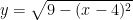 . But we’ll want to change the x to
  . All that means is the distance that you go from one disk, or one layer, of your water to the next. If we make this change, that tells us
 , this tells us that
 , we just have to multiply the mass of the ith layer by 9.8 to get the force acting on the ith layer.
 total meters. That tells us that the upper bound is going to be 7.
  . So, we know that it would take
  . Since it’s never fine to divide by zero, this isn’t allowed.
 in our new limit. But we’ll take the limit of a different function. And hopefully this one will be easier to evaluate.
 or
or  .
.  as
as  .
.
 ,
,  . Or $$\lim_{x \to 0^-} \ \frac{ – \ \frac{1}{1-x} \ – \ cos(x) }{ 2cos(x) \cdot sin(x) }=-\infty$$
 ,
,  . Or $$\lim_{x \to 0^+} \ \frac{ – \ \frac{1}{1-x} \ – \ cos(x) }{ 2cos(x) \cdot sin(x) }=\infty$$
 and the right-sided limit is
  can be tricky at first glance. I’m sure you’re probably familiar with how to take the
  part of it. In general, you’ll just want to remember that $$\int e^x \ dx = e^x$$
 piece looks a little weird. At first glance it may even look completely foreign. What have you seen that looks like this piece of the function?
 . We know that
  . So when we are trying to integrate the