Is Cady Right, or Does the Limit Exist?

I recently watched the movie Mean Girls. At the end of the movie, there is a scene where the main character is shown a limit and asked to evaluate it. After quickly working out the problem in a tight competition for the academic decathlon, Cady looks up from her paper and shouts, “THE LIMIT DOES NOT EXIST!”

And of course, being the math oriented person that I am, I just was left wondering whether the limit actually exists after Mean Girls concluded. So I figured I’d share my findings.

First of all, here’s the limit shown at the end of Mean Girls: $$\lim_{x \to 0} \ \frac{ln(1-x) \ – sin(x)}{1-cos^2(x)}$$

Where do we start?

Typically when I’m evaluating limits, I like to assume that the function is continuous at the point we’re evaluating the limit and just plug it in. This usually doesn’t work, but it will frequently give us a hint as to which method we can use to evaluate it. This basically just takes advantage of the basic limit properties of limits if it works out. But we need to make sure we’re not causing any problems when we do this.

So let’s just start with plugging in zero for x in the function who’s limit we’re looking for.

$$ f(x) = \frac{ln(1-x) \ – sin(x)}{1-cos^2(x)}$$ $$f(0)=\frac{ln(1-0) \ – sin(0)}{1-cos^2(0)}$$ $$f(0)=\frac{ln(1-0) \ – sin(0)}{1- \big( cos(0) \big)^2}$$ $$f(0)=\frac{0 \ – 0}{1- 1} = \frac{0}{0}$$

Turns out, this doesn’t really work this time. Because we end up with the indeterminate form of \frac{0}{0}. Since it’s never fine to divide by zero, this isn’t allowed.

So, we’ll need to think of another way to evaluate this limit. But like I said before, the fact that we got this indeterminate form gives us a hint of how we can evaluate this limit properly. This indeterminate form actually is one of the conditions that tells us we can evaluate this limit using L’Hospital’s Rule.

L’Hospital’s Rule

Which means we can create a new limit. We will still have x \to 0 in our new limit. But we’ll take the limit of a different function. And hopefully this one will be easier to evaluate.

This new limit will actually just be made up of a fraction where the top of the fraction is just the derivative of the original numerator. And the bottom of this new faction is just the derivative of the denominator of the original fraction. So we know that $$\lim_{x \to 0} \ \frac{ln(1-x) \ – sin(x)}{1-cos^2(x)} \ = \ \lim_{x \to 0} \ \frac{\frac{d}{dx} \big[ ln(1-x) \ – sin(x) \big] }{\frac{d}{dx} \big[ 1-cos^2(x) \big] }$$

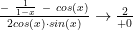
Remember, we are not finding the derivative of the fraction as a whole, so we should not use the quotient rule. We will need to apply the chain rule to find the derivative of a few of these terms. Doing so tells us that $$\lim_{x \to 0} \ \frac{ln(1-x) \ – sin(x)}{1-cos^2(x)} \ = \ \lim_{x \to 0} \ \frac{ – \ \frac{1}{1-x} \ – \ cos(x) }{ 2cos(x) \cdot sin(x) }$$

Now can we evaluate this limit?

The point of using L’Hospital’s Rule is that we should end up with a limit that’s easier to evaluate. So, let’s try the same thing we did earlier and see what happens. Since we have a limit as x \to 0, let’s just plug zero in for x and see what we get. $$\lim_{x \to 0} \ \frac{ – \ \frac{1}{1-x} \ – \ cos(x) }{ 2cos(x) \cdot sin(x) }$$ $$\frac{ – \ \frac{1}{1-(0)} \ – \ cos(0) }{ 2cos(0) \cdot sin(0)}$$ $$\frac{ – \ 1 \ – \ 1 }{ 2(1)(0)} = \frac{-2}{0}$$

And you can see we’ve divided by zero. So, this isn’t going to work. You can’t divide by zero, it breaks the rules of math. Therefore, we can’t just evaluate this limit by plugging in zero for x.

However, we are getting closer. The reason I say this is that we don’t have the indeterminate form of \frac{0}{0} anymore. Since we have some other number divided by zero, that tells us that this limit will likely be either \infty or - \infty.

The reason for this is that the numerator of the fraction is going toward the number -2. Whether you approach from the left or the right of x = 0, the top of our fraction is going to be a number close to -2.

Meanwhile, as x gets really, really close to 0, the denominator is going to also get really close to 0. But we don’t care about what the denominator is when x = 0. Since we’re dealing with a limit we care about the denominator when x is really close to 0. But depending on which side of zero we’re on, the denominator could be positive or negative.

If we have a fraction where the numerator is some non-zero number, and the denominator is getting infinitely close to zero, the fraction as a whole will become infinitely large. We just need to figure out if it’s positive or negative. Well, we can figure this out by splitting the limit up into two one-sided limits and see what those tell us about the two-sided limit.

Left-Sided Limit

Let’s start with the limit where x is approaching zero from the left. $$\lim_{x \to 0^-} \ \frac{ – \ \frac{1}{1-x} \ – \ cos(x) }{ 2cos(x) \cdot sin(x) }$$ We already know that the numerator of this fraction is going to approach -2 as x approaches 0 from either side. So, let’s just look at the denominator of this fraction.

What happens to 2cos(x)sin(x) as x \to 0? Well, we already said it will approach 0, but let’s just consider what’s going on as x approaches 0 from the left. If we’re approaching 0 from the left, that means we want to consider x values that are super close to 0, but will be negative. For negative x values approaching 0, cos(x) will approach 1, and will be slightly smaller than 1. And sin(x) will approach 0, and will be negative numbers very close to 0.

This is because sin(x) is negative for x values very close to 0. We can see this looking at a graph of f(x)=sin(x).

Graph of f(x) = sin(x)

Based on this, as x approaches 0, 2cos(x)sin(x) will become the product of 2, 1, and a negative number very close to 0. The product of two positive numbers and a negative number will be a negative number. So we know that this denominator will be getting closer and closer to 0, but will be a negative number in this left sided limit.

So we can think of the fraction as a whole, as a positive number very close to 2, divided by a negative number very close to 0. As x goes to 0 from the left, this fraction will get infinitely large and will be negative because it’s a positive divided by a negative. In other words, as x \to 0^-, \frac{ - \ \frac{1}{1-x} \ - \ cos(x) }{ 2cos(x) \cdot sin(x) } \to \frac{2}{-0}. Or $$\lim_{x \to 0^-} \ \frac{ – \ \frac{1}{1-x} \ – \ cos(x) }{ 2cos(x) \cdot sin(x) }=-\infty$$

Right-Sided Limit

The right-sided limit will work out very similarly, but with one main difference. $$\lim_{x \to 0^+} \ \frac{ – \ \frac{1}{1-x} \ – \ cos(x) }{ 2cos(x) \cdot sin(x) }$$ Again, the numerator of this fraction is going to approach -2 as x approaches 0 from the right. But let’s look at the denominator.

By the same process as the left-sided limit above, we can see that the denominator of this fraction is going to approach 0. But what we need to figure out is whether it is going to be approaching 0 from the negative side or the positive side. And the only term of our denominator that is going to be different approaching from the right side of 0, is sin(x).

Looking back up at the graph of f(x)=sin(x) you can see that the function is positive (above the x axis) to the right of x=0. Therefore, the denominator of this fraction is going to be the product of three positive numbers, resulting in a positive number. And the fraction as a whole will be a positive number over a positive number. In other words, as x \to 0^+, \frac{ - \ \frac{1}{1-x} \ - \ cos(x) }{ 2cos(x) \cdot sin(x) } \to \frac{2}{+0}. Or $$\lim_{x \to 0^+} \ \frac{ – \ \frac{1}{1-x} \ – \ cos(x) }{ 2cos(x) \cdot sin(x) }=\infty$$

What does this tell us about the two-sided limit?

Remember, for a limit to exist both one-sided limits need to exist AND they both need to be equal to each other. We just figured out that our left-sided limit is -\infty and the right-sided limit is \infty. Since one is positive and one is negative, they clearly aren’t equal. Each one-sided limit does not give the same result. Therefore, the limit we are trying to find indeed does not exist.

So, it turns out Cady was right in the end of Mean Girls. The limit does not exist.

Limits to Infinity

Limits as x approaches infinity can be tricky to think about. This is because infinity is not a number that x can ever be equal to. To evaluate a limit as x goes to infinity, we cannot just simply plug infinity in for x and see what we get. As a result, things like \mathbf{e^{\infty}} and \mathbf{\frac{1}{\infty}} don’t actually have a value.

So how can we deal with infinity?

Although infinity doesn’t have a specific value and can’t be plugged into functions, we can think about what will happen to a given function as x approaches infinity.

All this really means is that x is continually getting infinitely large. And as x gets bigger and bigger and bigger, what y value will our function get closer and closer to?

Let’s look at a few common examples and what they mean.

One Divided by Infinity

Like I said before, infinity is not a value. Therefore, \frac{1}{\infty} isn’t an actual number and doesn’t have a value. However, what we want to think about is what y value 1/x will approach as x goes to infinity. This is exactly what is being asked when we see: $$\lim_{x \to \infty} \frac{1}{x}$$

So let’s think about what happens to 1/x when we plug in bigger and bigger numbers for x.

x\mathbf{\frac{1}{x}}
11
100.1
1000.01
1,0000.001
10,0000.0001
100,0000.00001
1,000,0000.000001
10,000,0000.0000001
100,000,0000.00000001

So you can see in the table above that as x gets bigger and bigger, 1/x gets closer and closer to 0. Or in other words,

as x approaches infinity, 1/x approaches 0

We would write this mathematically as: $$\lim_{x \to \infty} \frac{1}{x} = 0$$

We can also see this graphically using Mathway. Notice in the graph below that as the x value goes toward infinity, you can see the y value getting closer to the y-axis (y=0).

limit as x goes to infinity of 1/x

Limits Going to Infinity

The other common example I mentioned is the limit as x goes to infinity of \mathbf{e^x}. Or $$\lim_{x \to \infty} e^x$$

Again, it doesn’t really make sense to say that we can just plug infinity in for x and get \mathbf{e^{\infty}}. This doesn’t actually have a value. This isn’t a number. Instead, we want to think about what y value \mathbf{e^x} goes toward as x goes to infinity. So let’s look at what happens as we raise e to a larger and larger power.

x\mathbf{e^x}
12.718
27.389
454.598
6403.429
82,980.958
1022,026.466
1002.688 * \mathbf{10^{43}}

So we can see here that \mathbf{e^x} starts giving us very large numbers quite quickly. And as we continue to plug in larger values for x, \mathbf{e^x} will continue to get bigger and bigger and bigger.

as x approaches infinity, \mathbf{e^x} approaches infinity

We would write this mathematically as: $$\lim_{x \to \infty} e^x = \infty$$

Rational Functions

Finding the limit as x approaches infinity of rational functions is a common limit you will run into. This is important because this is how you find horizontal asymptotes of rational functions. You are just looking to see what y value your function will get really close to (without touching that value) as your x goes to infinity.

What is a rational function?

A rational function is a function that is a fraction where the top and bottom of the fraction are polynomials. Basically this just means that the numerator and denominator of the fraction will be a sum of a handful of terms that are a constant times x raised up to some power. So it will look like this: $$f(x)=\frac{a_nx^n + a_{n-1}x^{n-1} + … + a_2x^2 + a_1x + a_0}{b_mx^m + b_{m-1}x^{m-1} + … + b_2x^2 + b_1x + b_0}$$

How do you take the limit of a rational function?

There are really only 3 cases you need to consider and the video above discusses these three cases as well. Any rational function will fall into one of these three categories, and each limit within each category will work out the same.

All you need to do is look at the degree of the polynomial on the top and bottom of the fraction. The degree of a polynomial is the highest power that x is being raised to. So for example, \mathbf{y=-4x^5+6x^2+x-12} is a polynomial of degree 5, because the highest power of x is 5.

Case 1: Degree of numerator is larger than degree of denominator

If the degree of the numerator is higher than the degree of the polynomial on the denominator, then the limit will go to infinity or negative infinity. This will only depend on the sign of the coefficient of the highest power x term on the numerator.

If Degree(P(x)) > Degree(Q(x)), then \mathbf{\lim\limits_{x \to \infty} \frac{P(x)}{Q(x)}= \pm \infty}

Example:

$$\lim_{x \to \infty} \frac{x^4-3x^2+x}{x^3-x+2}$$ $$=\lim_{x \to \infty} \frac{x^4-3x^2+x}{x^3-x+2} \cdot \frac{\frac{1}{x^3}}{\frac{1}{x^3}}$$ $$=\lim_{x \to \infty} \frac{\frac{x^4}{x^3}-\frac{3x^2}{x^3}+\frac{x}{x^3}}{\frac{x^3}{x^3}-\frac{x}{x^3}+\frac{2}{x^3}}$$ $$=\lim_{x \to \infty} \frac{x-\frac{3}{x}+\frac{1}{x^2}}{1-\frac{1}{x^2}+\frac{2}{x^3}}$$ $$= \frac{\lim\limits_{x \to \infty}x-\lim\limits_{x \to \infty}\frac{3}{x}+\lim\limits_{x \to \infty}\frac{1}{x^2}}{\lim\limits_{x \to \infty}1-\lim\limits_{x \to \infty}\frac{1}{x^2}+\lim\limits_{x \to \infty}\frac{2}{x^3}}$$ $$= \frac{\lim\limits_{x \to \infty}x-0+0}{1-0+0}$$ $$=\frac{\lim\limits_{x \to \infty}x}{1}$$ $$=\lim_{x \to \infty}x$$ $$=\infty$$

Case 2: Degree of numerator is smaller than degree of denominator

If the degree of the numerator is smaller than the degree of the denominator then the limit will go to 0.

If Degree(P(x)) < Degree(Q(x)), then \mathbf{\lim\limits_{x \to \infty} \frac{P(x)}{Q(x)}= 0}

Example:

$$\lim_{x \to \infty} \frac{16x^4}{0.0001x^5+18x}$$ $$=\lim_{x \to \infty} \frac{16x^4}{0.0001x^5+18x} \cdot \frac{\frac{1}{x^5}}{\frac{1}{x^5}}$$ $$=\lim_{x \to \infty} \frac{\frac{16x^4}{x^5}}{\frac{0.0001x^5}{x^5}+\frac{18x}{x^5}}$$ $$=\lim_{x \to \infty} \frac{\frac{16}{x}}{0.0001+\frac{18}{x^4}}$$ $$= \frac{\lim\limits_{x \to \infty}\frac{16}{x}}{\lim\limits_{x \to \infty}0.0001+\lim\limits_{x \to \infty}\frac{18}{x^4}}$$ $$= \frac{0}{0.0001+0}$$ $$=0$$

Case 3: Degree of numerator is equal to degree of denominator

If the degree of the numerator is equal to the degree of the denominator then the limit will be equal to the coefficient of the highest power x term in the numerator divided by the coefficient of the highest power x term in the denominator.

If Degree(P(x)) = Degree(Q(x)), then \mathbf{\lim\limits_{x \to \infty} \frac{P(x)}{Q(x)}= \frac{a}{b}} \ 
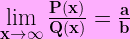
where a is the coefficient of the highest power x term in P(x), and b is the coefficient of the highest power x term in Q(x).

$$\lim_{x \to \infty} \frac{x^2+7}{-3x^2}$$ $$=\lim_{x \to \infty} \frac{x^2+7}{-3x^2} \cdot \frac{\frac{1}{x^2}}{\frac{1}{x^2}}$$ $$=\lim_{x \to \infty} \frac{\frac{x^2}{x^2} + \frac{7}{x^2}}{\frac{-3x^2}{x^2}}$$ $$=\lim_{x \to \infty} \frac{1 + \frac{7}{x^2}}{-3}$$ $$= \frac{\lim\limits_{x \to \infty}1 + \lim\limits_{x \to \infty}\frac{7}{x^2}}{\lim\limits_{x \to \infty}-3}$$ $$= \frac{1+0}{-3}$$ $$=-\frac{1}{3}$$

Other Examples

\mathbf{\lim\limits_{x \to \infty} arctan \big( e^x \big)} | Solution

\mathbf{\lim\limits_{x \to \infty} \frac{sin(x)}{x}} | Solution

\mathbf{\lim\limits_{x \to \infty} \frac{ln(x)}{\sqrt{x}}} | Solution

Solutions

Example 1 Solution

\mathbf{\lim\limits_{x \to \infty} arctan \big( e^x \big)}

This is going to be based on the fact that we already discussed above that \mathbf{\lim\limits_{x \to \infty} e^x = \infty}
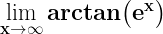
. Since we know that, we can say that \mathbf{y=e^x} and rewrite our limit as: $$\lim_{y \to \infty} arctan(y)$$

This is because y goes to infinity as x goes to infinity since \mathbf{y=e^x}. Now we can find this limit by looking at a graph of y=arctan(x).

limit as x approaches infinity of arctan(x) or tan^{-1}(x)

Looking at this graph we can see that y=arctan(x) has a horizontal asymptote at \mathbf{y=\frac{\pi}{2}}. As x goes toward infinity, you can see that the y value of our function gets closer and close to \mathbf{\frac{\pi}{2}}. So this tells us $$\lim_{y \to \infty} arctan(y)=\frac{\pi}{2}$$ $$\lim_{x \to \infty} arctan \big( e^x \big)=\frac{\pi}{2}$$

Example 2 Solution

\mathbf{\lim\limits_{x \to \infty} \frac{sin(x)}{x}}

This one is going to use Squeeze Theorem. Click here to learn more about Squeeze Theorem and its required conditions if you don’t already know about them, then come back to this problem.

We know that \mathbf{-1 \leq sin(x) \leq 1} for all x. Since we are looking at this limit as x goes to positive infinity, we can also say that $$-\frac{1}{x} \leq \frac{sin(x)}{x} \leq \frac{1}{x}$$

We also know that \mathbf{\lim\limits_{x \to \infty} -\frac{1}{x}=0} and that \mathbf{\lim\limits_{x \to \infty} \frac{1}{x}=0}. Since we know \mathbf{\frac{sin(x)}{x}} is between \mathbf{-\frac{1}{x}} and \mathbf{\frac{1}{x}} we can use Squeeze Theorem to say that $$\lim_{x \to \infty} \frac{sin(x)}{x}=0$$

Example 3 Solution

\mathbf{\lim\limits_{x \to \infty} \frac{ln(x)}{\sqrt{x}}}

For this limit, we will be able to use L’Hospital’s Rule. This is because ln(x) and \mathbf{\sqrt{x}} both go to infinity as x goes to infinity. This gives us an indeterminate form that is a possible application of L’Hospital’s Rule. We can also check to make sure that this meets the other conditions needed to apply L’Hospital’s Rule.

$$\lim_{x \to \infty} \frac{ln(x)}{\sqrt{x}}$$ $$=\lim_{x \to \infty} \frac{\frac{d}{dx}ln(x)}{\frac{d}{dx}\sqrt{x}}$$ $$=\lim_{x \to \infty} \frac{\frac{1}{x}}{\frac{1}{2x^{1/2}}}$$ $$=\lim_{x \to \infty} \frac{1}{x} \cdot \frac{2x^{1/2}}{1}$$ $$=\lim_{x \to \infty} \frac{2}{x^{1/2}}$$ $$=\lim_{x \to \infty} \frac{2}{\sqrt{x}}$$ $$=0$$

LIMIT PROPERTIES – Examples of using the 8 properties

I’ve already talked a bit about limits and one-sided limits and how to evaluate them, especially using the graph of the functions. But most limits that you need to evaluate won’t come with a graph and may be challenging to graph. In cases like these, you will want to try applying the 8 basic limit properties.

Using the limit properties is the simplest way to evaluate limits. Therefore, applying limit properties should be a good starting place for most limits. These properties can be applied to two-sided and one-sided limits.

First I will go ahead and list the 8 limit properties then I will show you a handful of examples that show how to apply these limits. These are the same 8 limit properties that are listed on my calculus 1 study guide. If you haven’t already, click here to download my calculus 1 study guide so you can have these limit properties handy as you work through evaluating limits with them.

What are the 8 limit properties?

\mathbf{1. \ \ \lim\limits_{x \to a} c = c}

Taking the limit of a constant just results in that constant.

\mathbf{2. \ \ \lim\limits_{x \to a} x = a}

The limit of the variable alone will go toward the value that the variable is approaching as given in the limit. This is a result of the fact that y=x is a continuous function.

\mathbf{3. \ \ \lim\limits_{x \to a} \Big( cf(x) \Big) = c \cdot \lim\limits_{x \to a} f(x)}

Having a constant being multiplied by the entire function within the limit can be pulled out of the limit. This will allow you to evaluate the simpler function, then multiply the result by that constant after evaluating a slightly simpler limit.

\mathbf{4. \ \ \lim\limits_{x \to a} \Big( f(x) \pm g(x) \Big) = \lim\limits_{x \to a} f(x) \pm \lim\limits_{x \to a} g(x)}

The limit of a sum or difference can instead be written as the sum or difference of their individual limits.

\mathbf{5. \ \ \lim\limits_{x \to a} \Big( f(x) \cdot g(x) \Big) = \lim\limits_{x \to a} f(x) \cdot \lim\limits_{x \to a} g(x)}

The limit of a product can instead be written as the product of their individual limits.

\mathbf{6. \ \ \lim\limits_{x \to a} \Big( \frac{f(x)}{g(x)} \Big) = \frac{\lim\limits_{x \to a} f(x)}{\lim\limits_{x \to a} g(x)}, \ \ if \ \lim\limits_{x \to a} g(x) \neq 0}

Taking the limit of a quotient can be rewritten as the quotient of those two limits. Just make sure that the limit of the denominator isn’t zero. If it is, then this will result in dividing by zero, which you can’t do.

\mathbf{7. \ \ \lim\limits_{x \to a} \Big( f(x) \Big)^n = \Big( \lim\limits_{x \to a} f(x) \Big)^n}

Taking the limit of some function raised to a constant power can be rewritten to evaluate the limit of the inner function then raise the result to that constant power.

\mathbf{8. \ \ \lim\limits_{x \to a} \Big( \sqrt[\leftroot{-3}\uproot{3}n]{f(x)} \Big) = \sqrt[\leftroot{-3}\uproot{3}n]{\lim\limits_{x \to a} f(x)}}

Similar to the last property, but the same can be done with a function that is within a root. This can be applied to any constant root (eg. square root, cube root, etc.)

How can these limit properties be applied to evaluate limits?

These 8 properties of limits can be used to simplify limits and break them down into smaller pieces. Each of these smaller pieces would be easier to deal with. Then once you evaluate these smaller, simpler limits you can put them all together.

We will go ahead and show how to apply these limit properties with some examples. To the right of each step in parenthesis, I will put a number corresponding to the property from above that was used to get to that step from the previous one. If multiple properties were applied at the same time I will list all properties used in that step in the parenthesis.

Example 1

$$\lim_{x \to 5} 6x^4 – 2x + 7$$ $$= \ \lim_{x \to 5} 6x^4 – \lim_{x \to 5} 2x + \lim_{x \to 5} 7 \ \ \ \ (4)$$ $$= \ 6 \lim_{x \to 5} x^4 – 2 \lim_{x \to 5} x + \lim_{x \to 5} 7 \ \ \ \ (3)$$ $$= \ 6 \Big( \lim_{x \to 5} x \Big)^4 – 2 \lim_{x \to 5} x + \lim_{x \to 5} 7 \ \ \ \ (7)$$ $$= \ 6 (5)^4 – 2(5) + 7 \ \ \ \ (1, \ 2)$$ $$= \ 3,747$$

Example 2

$$\lim_{x \to 2} \Big( (x+2) \sqrt[\leftroot{-1}\uproot{3}3]{x^2 + 7x} \Big)$$ $$= \ \lim_{x \to 2}(x+2) \cdot \lim_{x \to 2}\sqrt[\leftroot{-1}\uproot{3}3]{x^2 + 7x} \ \ \ \ (5)$$ $$= \ \Big( \lim_{x \to 2}x+ \lim_{x \to 2}2 \Big) \cdot \lim_{x \to 2}\sqrt[\leftroot{-1}\uproot{3}3]{x^2 + 7x} \ \ \ \ (4)$$ $$= \ (2+2) \cdot \lim_{x \to 2}\sqrt[\leftroot{-1}\uproot{3}3]{x^2 + 7x} \ \ \ \ (1, \ 2)$$ $$= \ 4 \lim_{x \to 2}\sqrt[\leftroot{-1}\uproot{3}3]{x^2 + 7x}$$ $$= \ 4 \sqrt[\leftroot{1}\uproot{3}3]{\lim_{x \to 2} \Big(x^2 + 7x \Big)} \ \ \ \ (8)$$ $$= \ 4 \sqrt[\leftroot{1}\uproot{3}3]{\lim_{x \to 2} x^2 + \lim_{x \to 2} 7x} \ \ \ \ (4)$$ $$= \ 4 \sqrt[\leftroot{1}\uproot{3}3]{\Big( \lim_{x \to 2} x \Big)^2 + 7 \lim_{x \to 2} x} \ \ \ \ (7, \ 3)$$ $$= \ 4 \sqrt[\leftroot{1}\uproot{3}3]{(2)^2 + 7(2)} \ \ \ \ (2)$$ $$= \ 4 \sqrt[\leftroot{-1}\uproot{1}3]{18}$$

Example 3

$$\lim_{x \to 4} \frac{x}{28}$$ $$= \ \frac{\lim\limits_{x \to 4} x}{\lim\limits_{x \to 4} 28} \ \ \ \ (6)$$ $$= \ \frac{4}{28} \ \ \ \ (1, \ 2)$$ $$= \ \frac{1}{7}$$

Conclusion

As you can see, each of these properties can be applied to fairly complex limits to break them down into smaller, simpler pieces. Each will usually end in applying one of the first two properties listed above to convert a limit into some number. And in the end, you will end up converting all of the limits into numbers. At that point, you will be able to manipulate everything with simple algebra to simplify your answer.

If you’d like to get your own copy of my FREE STUDY GUIDE, you can get yours by clicking here. And check out and subscribe to my YouTube Channel as well for video versions of other topics that I have posted lessons about as well.

L’HOSPITAL’S RULE – HOW TO – With Examples

L’Hospital’s Rule really just tells us one thing that makes evaluating certain limits a lot easier. Limits that meet 3 specific requirements can be made much simpler using L’Hospital’s Rule. First let me introduce L’Hospital’s Rule, then we can go over the 3 conditions that you need to check before you can apply it to any given limit.

What does L’Hospital’s Rule tell us?

To find a limit of a function that is a fraction, we can take the derivative of the top of the fraction and the derivative of the bottom of the fraction and make a new fraction out of the derivatives.

$$\lim_{x \to a} \frac{f(x)}{g(x)} = \lim_{x \to a} \frac{f'(x)}{g'(x)}$$

Notice that we don’t use the quotient rule here. The reason for this is that we are taking the limit of this fraction and not taking the derivative of this fraction. The limit is the key piece that allows us to avoid the quotient rule and take the derivative of each piece of the fraction separately to create another limit that is equal to the original.

The hope is that the fraction resulting from the derivatives will be easier to evaluate than the original limit was.

How do we know when to use L’Hospital’s Rule?

Before we can apply L’Hospital’s rule to any given limit, we need to confirm that these three conditions are met:

  1. f(x) and g(x) are differentiable on some open interval that includes \mathbf{x=a}. This will basically just mean that both the numerator and denominator are differentiable at x=a.
  2. \mathbf{g'(x) \neq 0} near \mathbf{x=a}. Note that it doesn’t matter if g'(x)=0 AT x=a as long as you can pick some interval (as small as is necessary) around x=a where g'(x) \neq 0 for all x‘s in that interval besides x=a. You likely won’t need to worry about running into a function that you can’t pick a small enough interval around x=a to make this work.
  3. As x \rightarrow a, f(x) AND g(x) \mathbf{\rightarrow 0} — OR — f(x) AND g(x) \mathbf{\rightarrow \pm \infty}

That’s really all there is to it. Let’s jump into some practice problems and I will show you how to apply L’Hospitals Rule.

Example 1

Evaluate the following limit using L’Hospital’s Rule or explain why L’Hospital’s Rule cannot be used to evaluate this limit.

$$\lim_{x \to \infty} \frac{e^x}{-x^2+1000x}$$

If we tried to use limit properties to evaluate this limit, we would see that both the top and the bottom of this fraction go to either positive or negative infinity as x goes to infinity.

$$\lim_{x \to \infty} \frac{e^x}{-x^2+1000x} \rightarrow \frac{\infty}{- \infty}$$

So L’Hospital’s Rule might help…

Now we just need to confirm that the other two conditions are met.

f(x)=e^x is an exponential function and is differentiable everywhere, for any value of x. And g(x)=-x^2 + 1000x is also differentiable everywhere since it’s a polynomial. Since it’s differentiable everywhere, it is also differentiable for any infinitely large x value.

g'(x) = -2x+1000 will go to -\infty as x approaches \infty. g'(x) \neq 0 for any infinitely large x value since it just continues to go to - \infty.

So we know that this limit meets all 3 requirements needed to apply L’Hospital’s Rule.

Now we know we can apply L’Hospital’s Rule

Taking the derivative of the top and bottom of the fraction individually tells us that:

$$\lim_{x \to \infty} \frac{e^x}{-x^2+1000x} = \lim_{x \to \infty} \frac{e^x}{-2x+1000}$$

Now we can evaluate this new limit instead. But if we do this, we will notice that we will still end up in the same situation that we had before.

$$\lim_{x \to \infty} \frac{e^x}{-2x+1000} \rightarrow \frac{\infty}{- \infty}$$

But what if it didn’t really help make the limit easier?

Which puts us in a perfect situation to consider using L’Hospital’s Rule to evaluate this new limit as well. By the same logic as before, we can confirm that the first two conditions are met as well as x gets infinitely large. Since all 3 required conditions are met we can go ahead and apply L’Hospital’s Rule a second time.

$$\lim_{x \to \infty} \frac{e^x}{-2x+1000} = \lim_{x \to \infty} \frac{e^x}{-2}$$

Now we can simply use the basic limit properties to evaluate this last limit.

Now we have a much easier limit

$$\lim_{x \to \infty} \frac{e^x}{-2} = \ – \frac{1}{2} \lim_{x \to \infty} e^x = \ – \infty$$

So therefore,

$$\lim_{x \to \infty} \frac{e^x}{-x^2+1000x} = \ – \infty$$

A quick note on applying L’Hospital’s Rule twice

This is an interesting problem because it shows that you can apply L’Hospital’s Rule multiple times on the same problem. You just need to make sure that each time you apply it, the resulting limit still meets all 3 required conditions before applying it to the new limit. There is no limit to the number of times you can continue applying L’Hospital’s Rule over and over in the same problem as long as you are making sure that the limit you are applying it to meets all 3 conditions every time you apply it.

Example 2

Evaluate the following limit using L’Hospital’s Rule or explain why L’Hospital’s Rule cannot be used to evaluate this limit.

$$\lim_{x \to 3} \frac{x-3}{27-x^3}$$

Again, if we think about what value the top and bottom of this fraction will go towards as x approaches 3, we would see that

$$\lim_{x \to 3} \frac{x-3}{27-x^3} \rightarrow \frac{0}{0}$$

Since we get another indeterminate form, which is $\frac{0}{0}$, we should consider using L’Hospital’s Rule to make this limit easier to evaluate.

So L’Hospital’s Rule might help…

First, we need to make sure that the other two conditions are met as well.

We can check that g'(x) = -3x^2 doesn’t equal zero anywhere near x=3. This is because g'(x) = -3x^2 is continuous everywhere and the only place where g'(x)=-3x^2=0 is when x=0. As a result of these two things, we can pick some interval around x=3 that doesn’t include x=0 to satisfy condition #2.

Also, both f(x) and g(x) are polynomials and are therefore differentiable everywhere. So we know they will both be differentiable on any interval around x=3.

Now we know we can apply L’Hospital’s Rule

Doing so by taking the derivative of the top and bottom of our fraction separately tells us that

$$\lim_{x \to 3} \frac{x-3}{27-x^3} = \lim_{x \to 3} \frac{1}{-3x^2}$$

And doing this gives us an easier limit to deal with. Now we can simply apply the limit properties to evaluate. Applying the limit properties tells us that:

$$\lim_{x \to 3} \frac{1}{-3x^2} = \frac{1}{-3 \Big( \lim_{x \to 3}x \Big) ^2}= \frac{1}{-3(3)^2} = \ – \frac{1}{27}$$

So therefore we know that:

$$\lim_{x \to 3} \frac{x-3}{27-x^3} = \ – \frac{1}{27}$$

Example 3

Evaluate the following limit using L’Hospital’s Rule or explain why L’Hospital’s Rule cannot be used to evaluate this limit.

$$\lim_{x \to 0} \frac{|x|}{x^5+2x}$$

If we think about what value the numerator and denominator of this fraction will approach as x approaches 0 from both sides, we would see:

$$\lim_{x \to 0} \frac{|x|}{x^5+2x} \rightarrow \frac{0}{0}$$

Since we get an indeterminate form, which is $\frac{0}{0}$, we should consider using L’Hospital’s Rule to make this limit easier to evaluate.

So L’Hospital’s Rule might help…

First, we need to make sure that the other two conditions are met as well.

Upon checking condition #1 however, we run into a problem. Condition #1 requires that f(x) and g(x) are both differentiable on some interval containing x=0, including x=0.

But f(x) = |x| is not differentiable at x=0. Therefore, we actually can’t apply L’Hospital’s Rule to evaluate this limit. I won’t go into the details here since we won’t be using L’Hospital’s Rule. But if you want to try evaluating this limit, I’d recommend considering both one-sided limits on their own and compare them to start. You can see a similar application here.

Example 4

\mathbf{\lim\limits_{x \to \infty} \frac{ln(x)}{\sqrt{x}}} | Solution

Solution – Find the values of a and b that make f continuous everywhere

Consider the following piecewise function: $$f(x) = \begin{cases} \frac{x^2-4}{x-2} & \mbox{if } x<2 \\ ax^2-bx+3 & \mbox{if } 2\leq x<3 \\ 2x-a+b & \mbox{if } x\geq 3 \end{cases}$$

Jake’s Math Lessons Complete Calculus 1 Package


Problem credit: Chapter 2.4 #36 in Single Variable Calculus: Concepts and Contexts by James Stewart.

How to find a and b for a piecewise function to be continuous everywhere.

When we see piecewise functions like this and our goal is to make sure it is continuous everywhere, there are two cases we want to consider separately:

  1. making each individual piece continuous on its reduced domain,
  2. and making the different pieces line up when our function switches between them.

First let’s consider each piece individually on the reduced domain where f is actually defined by that function.

Piece 1: y=\frac{x^2-4}{x-2} when x<2

When considering a function to find x values where the function is not continuous, two very common things to look for would be taking the square root of a negative number or dividing by zero.  Obviously we don’t need to worry about taking the square root of a negative number here since we don’t have any square roots.  However, we do have a fraction, and therefore we should consider if there is an x value that would cause us to divide by zero.

Looking at the denominator of our fraction, we see that we would divide by zero when we plug in some number for x that causes

$$x-2=0.$$

Clearly, this would happen when x=2.  And in fact, this is the only value for x where y=\frac{x^2-4}{x-2} is not continuous.  However, remember that I said we want to see if there are any x values that cause the function not to be continuous within our limited domain for the specific piece of the function.  Since x=2 is NOT in the domain x<2, we can say that this piece of our function is continuous on its entire domain and won’t contribute any discontinuities to f.

Piece 2: y=ax^2-bx+3 when 2\leq x<3

Looking at this piece of our piecewise function, clearly we need to consider our constants a and b.  Since our function f is a function of x (indicated by f(x)), we can consider the other letters in this piece of our function (a and b) to be constants.  I discussed this in a bit more detail here, but it basically means that a and b are some set number, they do not change.

The important thing to realize though, is that regardless of what values we choose for a and b, this piece of our function will just be a polynomial.  More specifically, it will be a quadratic function.  No matter what our a and b end up being we will have an x^2 term, an x term, and a constant term.  Since we know this piece of our function will be a polynomial no matter what our a and b are we can say that this piece of our function will be continuous for any a and b we select.

This is the case because polynomials are always continuous everywhere.  If this section of our function would be continuous everywhere, it would certainly be continuous on our limited domain of 2\leq x<3.  Therefore, we don’t need to worry about our a and b causing any discontinuities here.

Piece 3: y=2x-a+b when x\geq 3

This is actually going to be similar to piece 2 above.  We can see by looking at this function that no matter what a and b values we select here, they will both be constants which will combine to a single constant when we combine like terms.  Once we do this, we will be left with an x term and a constant term.  Therefore, this is also a polynomial (in this case it would also be a linear function), and would be continuous everywhere as a result.  Because of this, it must be continuous on our limited domain of x\geq 3.

Now we have shown that we will not get any discontinuities within any of our restricted domains that make up our piecewise function, but what about on their edges.  We also have to make sure we are selecting an a and a b value so that we can switch from one part of our function to the other without jumping up or down and leaving a hole in our function.  If we do not select the correct a and b we may get discontinuities at the x values where we switch from one function to the other.

In order to prevent this, we need to make sure that our first two pieces of f(x) transition smoothly when x=2 (this is the place we switch between these two functions) and we need to make sure that the second and third piece of our function have a smooth transition between them at x=3.

Continuity at x=2

Remember by definition, a function f(x) is continuous at x=a if $$\lim_{x \to a} f(x) = f(a).$$

We need to apply this rule here to make sure that our function f is continuous at x=2. Therefore, we need to pick an a and a b so that $$\lim_{x \to 2} f(x) = f(2).$$

As I explained here, a limit will only exist if both of its one-sided limits exist and are equal to each other.  Therefore, rather than finding the above limit, we actually want to find these two one-sided limits:

$$\lim_{x \to 2^{-}} f(x) = f(2)$$

$$\lim_{x \to 2^{+}} f(x) = f(2).$$

Let’s start with the left-sided limit.  Since we are approaching x=2 from the left, we are looking at x values that are slightly less than 2.  Therefore, we need to use the piece of our function that is defined for x<2.  So the limit we really want to find, and the equation we want to solve is:

$$\lim_{x \to 2^{-}} \frac{x^2-4}{x-2} = f(2).$$

When attempting to solve this limit, we see that we can not just plug in 2 for x because this would cause us to divide by zero.  As a result of this, I would first suggest simplifying the function whose limit we are trying to find.  Using the difference of squares rule on the top of our fraction we can rewrite this limit as

$$\lim_{x \to 2^{-}} \frac{(x+2)(x-2)}{x-2} = f(2).$$

Once we do this, we can see that the top and bottom of our fraction contain a (x-2) term so we can use them to cancel each other out.  This leaves us with

$$\lim_{x \to 2^{-}} (x+2) = f(2).$$

y=x+2 is a linear function and is continuous everywhere, so we can simply plug in x=2 to find this limit.

$$4=f(2)$$

Now we need to figure out the right side of the equation.  To find f(2), we just need to plug in x=2 into our function f(x), which is our original piecewise function.  The first thing we need to do is decide which piece defines our function when x=2.  We know that f(x)=ax^2-bx+3 when 2\leq x<3.  We can use this part to find f(2) because this is the piece that defines f when x=2.  Plugging in 2 for x we get

$$4=ax^2-bx+3$$

$$4=a(2)^2-b(2)+3$$

$$4=4a-2b+3$$

$$1=4a-2b$$

Notice we have only one equation at this point which relates two unknown constants, making it impossible to find one unique solution for a and b.  To do this we will need another equation relating these two constants.

I would also like to point out that this equation came from using the equation involving only the left sided limit, and we still need to look at the right sided limit.

$$\lim_{x \to 2^{+}} f(x) = f(2)$$

If we look at this limit, we see that we would be approaching x=2 from the right side, which would mean we are looking at x values slightly larger than 2.  For x values slightly larger than 2, but infinitely close to 2, we would use the y=ax^2-bx+3 piece to define f.  We already found f(2) above, so putting these two facts together we see

$$\lim_{x \to 2^{+}} ax^2-bx+3 = a(2)^2-b(2)+3$$

Since the function whose limit we are trying to find is continuous everywhere (since it’s a polynomial) we can just plug in 2 for x to find this limit.

$$a(2)^2-b(2)+3=a(2)^2-b(2)+3$$

$$4a-2b+3=4a-2b+3$$

Notice both sides of this equation are the same.  Because of this, this equation will actually be true no matter what we put in for a and b.  This doesn’t really help us at all in this case, but it was important to test it out and see what it told us.  So we know that f will be continuous at x=2 as long as

$$1=4a-2b.$$

At this point we have found a set of a and b values that make f continuous at x=2.  But we need to find just one a and one b that will accomplish this for all x values.

But this does not tell us anything about whether it would also be continuous at x=3.  Checking that may give us another relationship between a and b that we can use to find the single unique solution for the two constants that will make f continuous everywhere.

Continuity at x=3

Making sure that f is continuous at x=3 will be an extremely similar process to what we just did around x=2.  Similar to above, we will need to make sure the following equations are true:

$$\lim_{x \to 3^{-}} f(x) = f(3)$$

$$\lim_{x \to 3^{+}} f(x) = f(3).$$

Let’s start with the right sided limit.  This means that we are getting closer and closer to x=3 and we are coming from x values that are slightly larger than 3.  Therefore, we will need to use the piece of our function that defines f for x\geq 3.

$$\lim_{x \to 3^{+}} 2x-a+b = f(3)$$

Since a and b are both constants, y=2x-a+b is a linear function, and is continuous everywhere as a result.  Because of this, we can just plug 3 in for x to find this limit.

$$2(3)-a+b = f(3)$$

$$6-a+b = f(3)$$

To find f(3) we just need to plug 3 in for x into the piece of our function that defines it when x=3, which is the third piece of f.

$$6-a+b = 2(3)-a+b$$

$$6-a+b = 6-a+b$$

We see here another case where this equation gives us no useful information.  This is because this equality will be true no matter what we plug in for a and b.  Let’s move onto the left sided limit and see what we get there.

$$\lim_{x \to 3^{-}} f(x) = f(3)$$

Now that our x value is approaching 3 from the left side, it is slightly smaller than 3 and slowly increasing.  Since we are considering what our function is doing around x=3 for x values slightly smaller than 3, we will want to use the piece of f that is defined for 2\leq x<3.  We already found f(3) above, so we will also plug that in.

$$\lim_{x \to 3^{-}} ax^2-bx+3 = 6-a+b$$

Just like before, since we know y=ax^2-bx+3 is a polynomial, it is continuous everywhere and we can find this limit by plugging in x=3.

$$a(3)^2-b(3)+3 = 6-a+b$$

$$9a-3b+3 = 6-a+b$$

$$10a-4b=3$$

Putting it all together

Now we have another relationship that relates a and b.  Alone, it isn’t very useful, but we can take the previous equation we found from ensuring f is continuous at x=2 and solve the following system of equations:

$$\mbox{(1):         }4a-2b=1$$

$$\mbox{(2):         }10a-4b=3.$$

Now that we have two equations that relate these two unknown constants, we have enough information to solve for them.  You always need at least as many equations as you have variables (or unknown constants in this case).  There are a couple different ways to solve a system of equations like this, but I will use substitution.  First we will solve for b in equation (1), then plug that into equation (2).

$$4a-2b=1$$

$$-2b=-4a+1$$

$$\mbox{(3):         }b=2a-\frac{1}{2}$$

Now we will plug this into equation (2) and solve for a.

$$10a-4\Big(2a-\frac{1}{2}\Big)=3$$

$$10a-8a+2=3$$

$$2a+2=3$$

$$2a=1$$

$$a=\frac{1}{2}$$

Now we can plug this back into our equation for b, equation (3).

$$b=2\Big(\frac{1}{2}\Big)-\frac{1}{2}$$

$$b=1-\frac{1}{2}$$

$$b=\frac{1}{2}$$

Now we have shown that f(x) will be continuous at x=2 and at x=3 if a=\frac{1}{2} and b=\frac{1}{2}.  We already showed that f is continuous for x<2, 2<x<3, and x>3 for all values of a and b.  Now we also know that f is continuous at x=2 and x=3 if a=\frac{1}{2} and b=\frac{1}{2}.  Therefore, we can say that f would be continuous everywhere if a=\frac{1}{2} and b=\frac{1}{2}.

In fact, we can see that f is continuous by plugging in the values we found for a and b and graphing it using Desmos.

find a and b for piecewise function to be continuous

This type of problem is one that you will likely run into a few times.  It actually comes in handy when you are trying to solve a similar type of problem that requires you to make a function differentiable everywhere.  If you would like to see this I have worked through one of these and you can see that by clicking this link: Solution – Find the values of a and b that make the function differentiable everywhere.

SHORTCUT – More examples

Check out the other topics I’ve covered and the problems I’ve worked through.  You can see a list of related lessons on my limits page.

Also, I can send you a copy of my calculus 1 study guide to help you boost your test scores. All you have to do is enter your name and email below and I’ll send it your way!

As always, please don’t forget to leave a comment or send me an email if you have any questions on this post!  You can email me at jakesmathlessons@gmail.com.  Also, if you have any suggested topics or problems for a future post, I’d love to hear them.

** DISCLAIMER: Some links in this post may be affiliate links meaning I would get a small commission for your purchase at no extra cost to you. **

Finding Derivatives with Limits

At this point we should have at least a basic understanding of limits and how to find some limits.  However, I have only really discussed limits by themselves and not how they relate to the rest of calculus.  They are very important in calculus because they are used to define the most important calculus topics.

For example, the main topic which will be discussed for quite some time is derivatives.  Derivatives will come up in a lot of different settings, like finding rate of change, instantaneous rate of change, velocity, slope, and a few others.  The main thing to realize is that a derivative is generally used to find out how quickly, or slowly, something is changing.

I will go further into all of these things later, but for now I want to focus on the definition of derivatives and how to find a derivative using the definition.

The definition of a derivative

If we have some function, f(x), we would write “the derivative of f” as f'(x).  And we would define the derivative of f by using this limit:

$$f'(x) = \lim_{h \to 0} \frac{f(x+h) – f(x)}{h}$$

This limit can be a bit confusing, so there’s something I would like to point out before we actually begin working with this limit.  The confusing thing here is that we have x and h in this limit and it looks as if they are both variables.  However, when we find this limit, we can only treat h as a variable.  We will need to treat x as a constant and h as the only variable.

The reason for this is that we are finding the limit as h goes to 0.  This tells us that h is moving in toward 0.  It does not tell us that x is changing at all.  Therefore, when we are working with the limit, we will act as if x is a number, or a constant.  This means that once we find the limit, our answer may have x in it still and this is completely fine since x isn’t the variable in this case.  Now let’s try an example.

Example 1

Consider the function f(x) = 4x^2 - 7x + 12.  We will use the limit definition to find the derivative of this function, but first let’s break it down and consider each part on its own.

Finding f(x+h)

The fist thing we need to find is f(x+h).  This notation basically just means that we need to look at our function f, and plug in (x+h) wherever we see the input.  In other words, we need to replace all of the x‘s in the function with (x+h)‘s.  So,

$$f(x+h) = 4(x+h)^2 – 7(x+h) + 12.$$

Then we will want to expand this out so it’s easier to work with.  Remember (x+h)^2 is the same as (x+h)(x+h), which means we need to foil it.

$$f(x+h) = 4(x+h)(x+h) – 7(x+h) + 12$$

$$=4(x^2 + xh + xh + h^2) – 7(x+h) + 12$$

$$=4(x^2 + 2xh+ h^2) – 7(x+h) + 12$$

$$=4x^2 + 8xh+ 4h^2 – 7x – 7h + 12$$

Since there aren’t any like terms we will leave it at that for now.

Putting it all together

Now we can put that into the rest of the equation.  Since we now know f(x+h) and f(x), we can plug those into the equation.  I would recommend surrounding each of them with a set of parenthesis so you don’t forget to distribute the negative sign in front of the f(x).  This is a very common mistake, so be careful not to forget that because it will give you the wrong answer.

$$f'(x) = \lim_{h \to 0} \frac{f(x+h) – f(x)}{h}$$

$$= \lim_{h \to 0} \frac{(4x^2 + 8xh+ 4h^2 – 7x – 7h + 12) – (4x^2 – 7x + 12)}{h}$$

Solving the limit

When I first see a limit, the first thing I usually consider is whether we can simply plug in 0 for h. Essentially, I try to treat this function as if it were continuous at h=0 (remember h is the variable here).

However, if we do this here we will get 0 on the denominator.  Since you cannot divide by 0, this will not work.  So our strategy will be to simplify this fraction to a point where we can plug in 0 for h.  The simplest way to do this is to rearrange the numerator so that we can cancel an h from the numerator and denominator and get rid of our fraction all together.

$$f'(x)= \lim_{h \to 0} \frac{4x^2 + 8xh+ 4h^2 – 7x – 7h + 12 – 4x^2 + 7x – 12}{h}$$

$$= \lim_{h \to 0} \frac{8xh+ 4h^2 – 7h}{h}$$

At this point I would like to point something out. Notice, after simplifying the numerator of the fraction, each term remaining contains an h in it.  This is important because it allows us to factor the h out and cancel it with the h in the denominator, getting rid of the fraction.  This will be an extremely common strategy to use for finding the derivative of a function using the limit definition.

$$f'(x)= \lim_{h \to 0} \frac{h(8x+ 4h – 7)}{h}$$

$$= \lim_{h \to 0} 8x+ 4h – 7$$

Now we have simplified to a point that we can solve this limit by plugging 0 in for h.

$$f'(x)= 8x+ 4(0) – 7$$

$$= 8x – 7$$

So we have just shown that if f(x)=4x^2-7x+12, then f'(x)=8x-7.  We will later learn shortcuts like the product rule, quotient rule, and chain rule that will make finding derivatives like this much simpler and faster, but you will need to know how to find these using the limit definition.  The pattern shown in this problem is a common one.  It won’t work for all derivatives, but it’s a good thing to try first.

  • It’s generally a good idea to see if you can reengage the top of the fraction in such a way that every term has h as a factor.
  • Then you can factor out the h, and cancel it with the h on the bottom of the fraction.
  • This usually leaves you with a function that you can directly plug 0 into h and simplify from there, leaving you with a function that doesn’t contain any h‘s, but usually contains x‘s.

Enter your email below and I’ll send you my calculus 1 study guide which is packed full of helpful tricks and shortcuts to help you boost your scores in calc!

I would recommend checking out the other material I have about derivatives.  As I mentioned before, there are several shortcuts and methods that make this whole process a lot easier.  Go check out what I’ve written about on the derivatives page.  If you have a question that isn’t answered there just let me know by emailing me at jakesmathlessons@gmail.com.  I’ll do my best to answer any questions you send me and I may even post a lesson or full solution on it!

Continuity

Continuity is a relatively simple concept, but problems that require proving it can be a little tricky. Essentially, a continuous function is one that you can draw all in one motion without picking up your pencil. This is one explanation of what it means for a function to be continuous that I like because it doesn’t take any mathematical definitions or proofs to understand. Any holes or gaps in a function’s graph would be a discontinuity and would mean that the function is not continuous.

The limit definition of continuity

By definition, a function f(x) is continuous at x=a if $$\lim_{x \to a} f(x) = f(a).$$

Let’s think about what this equation is saying. The left side of this equation is something that we’ve already dealt with, limits. It’s asking us to find out what y value we close in on as we travel along our function and close in on x=a. Keep in mind, x is a variable here which represents the input of our function, f(x), and a is a constant. This means that a represents some specific number, which could be any number.

The right side of the equation is simply asking us to plug that same a value into f(x) and take the y value we get out.

In total, the above equation says that if we travel along a function and close in on a specific x value, we should close in on the same y value we would get if we simply plugged that x value into the equation.

In other words, as we travel along a function toward a specific x value, our y value will also go toward the y value of the function at that point. If that is the case, then the function is continuous at that specific point. If we can say that a function is continuous at every single possible value we could put in for a, then we can say that the function is continuous for all x. If this is true then we can draw our entire function in one motion without picking up our pencil!

Let’s do a couple examples.

Example 1

Remember back in the first lesson about limits, Limits – Intro, I said I would go back to discussing the importance of our limit in the first example giving us the same value as when we plugged x=2 into the equation?  I would like to go into that further.

continuity
Figure 1.1

The function we were considering was f(x) = x^2 and we were finding

$$\lim_{x \to 2} x^2.$$

After looking at the graph of this function, shown in Figure 1.1, we saw that

$$\lim_{x \to 2} x^2 = 4.$$

I also pointed out that plugging in x=2 directly into the function also returns a y value of 4. In other words, we know $$f(2) = 4.$$ Therefore, we know

$$\lim_{x \to 2} x^2 = 4 = f(2)$$

$$\lim_{x \to 2} x^2 = f(2).$$

Notice this is exactly like the definition of what it means for a function to be continuous at a point. If you replace a with 2, replace f(x) with x ^2, and replace f(a) with 4, we have just shown that y=x^2 is a function that is continuous at x=2.

Example 2

The next example I want to discuss also goes back to a function we have already looked at. Referring back to Limits – Intro we will consider f(x) shown in Figure 1.2.

Figure 1.2

The question we will answer here is whether this function is continuous at x=1 or not. What do you think?

There are a few different ways we can answer this question. The simplest would be to simply look at the graph of the function and think about whether we can draw that function at and around x=1 without picking up our pencil. As you can see, there is clearly a hole at x=1 where we would need to pick up our pencil, and add a single point at (1, \ 4).

As a result, it is probably safe to say that this function is not continuous at x=1. However, we want to be able to show this using the actual definition of what it means for a function to be continuous.

Remember, for this function, which we are calling f(x) in this case, we need to be able to show that $$\lim_{x \to 1} f(x) = f(1).$$

If we can show this equation to be true, then f(x) is continuous at x=1, and if it’s not true then the function is not continuous at x=1. Luckily, back when I first used this function as an example in the Limits – Intro lesson, we found that $$\lim_{x \to 1} f(x) = 2.$$ Therefore, we just need to find out if f(1) is also 2 and we can prove that this function is continuous or not continuous.

Looking at the graph again, we see that this function has a hole at x=1 and includes the point (1, \ 4). In other words, if we plug 1 into f(x) as our x value, we get a y value of 4 out. This is the same as saying f(1) = 4.

Now, at this point we have figured out $$\lim_{x \to 1} f(x) = 2 \ and$$ $$f(1) = 4.$$

Therefore, $$\lim_{x \to 1} f(x) \neq f(1)$$ and we can say that f(x) is not continuous at x=1.

More Examples

Find the values of a and b that make f continuous everywhere.

$$f(x) = \begin{cases} \frac{x^2-4}{x-2} & \mbox{if } x<2 \\ ax^2-bx+3 & \mbox{if } 2\leq x<3 \\ 2x-a+b & \mbox{if } x\geq 3 \end{cases}$$

To see the solution to this problem, click here.

I also have a calc 1 study guide that you can get now for FREE! Just enter your name and email below and I’ll send you a copy straight to your inbox!

There are also several other lessons and problems on my limits page.  It would be a good idea to get some practice with limits.  A lot of other more complex topics in calculus are based around limits so they are important to understand.  If you can’t find the topic you want to read about just let me know by emailing me at jakesmathlessons@gmail.com and I’ll do my best to answer your question!

Squeeze Theorem

The Squeeze Theorem is a useful tool for finding complex limits by comparing the limit to two much simpler limits. Squeeze Theorem tells us that if we know these three things:

$$1. \ \ \ g(x) \leq f(x) \leq h(x)$$

$$2. \ \ \ \lim_{x \to a} g(x) = L$$

$$3. \ \ \ \lim_{x \to a} h(x) = L$$

Then we also know that

$$\lim_{x \to a} f(x) = L$$

Keep in mind, requirement number 1 above only needs to be true around x=a. It does not need to be true at x=a and it also does not need to be true when we get far away from x=a. This is because limits only care what is happening to a function when we get infinitely close to a given x value, not at that x value and certainly not far away from that x value.

Example 1

You will typically see this used when you are finding the limit of a function which is made up of two functions being multiplied together and one of them is a trig function. For example, consider

$$\lim_{x \to 0}x ^4 sin \bigg( \frac{1}{\sqrt{x}} \bigg).$$

At first glance, this limit looks terribly complicated. Especially because the function f(x) = x ^4 sin \Big( \frac{1}{\sqrt{x}} \Big) doesn’t even exist at x=0 (plugging in x=0 directly causes you to divide by 0, which can’t be done). However, if we use Squeeze Theorem, we can find this limit by finding two other limits that are much easier to find.

Squeeze Theorem says that we will need to find one function that is greater than or equal to f(x) around x=0 (because we are finding the limit as x \to 0) and another function that is less than or equal to f(x) around x=0. It is not always obvious which functions to use for comparison, but any function that is made up of sine or cosine of something multiplied by something else will usually follow the same pattern, so this is a good thing to try first.

What’s the pattern?

Consider the function y = sin(x). No matter what you plug in for x you will always get a y value between -1 and 1. This will be true regardless of what you are taking the sine of. Even if you were to take sin\Big( \frac{1}{\sqrt{x}} \Big). No matter what you put in for x this will give you something between -1 and 1, except if you try to put in x=0 (remember you can’t divide by 0).

But remember, with limits it doesn’t matter what happens at the x value we are approaching, only what is happening around that point. Therefore, it doesn’t matter that this function isn’t defined at x=0 because it is defined for all x values near x=0.

The point I’m trying to make is that sine of anything can be bound between -1 and 1, so we can say:

$$-1 \leq sin(x) \leq 1, \ and$$

$$-1 \leq sin \bigg( \frac{1}{\sqrt{x}} \bigg) \leq 1$$

How does this relate to our example?

Now, the trick that makes this whole thing work is the fact that multiplying both sides of an inequality by a positive number maintains the inequality. Therefore, we can also multiply both sides of the inequality by a function that always outputs a positive number (or 0).

For example, we can multiply both sides by x^4, or all three “sides” in this case. We can do this because any number raised to an even power will always be positive (or 0). This gives us

$$x^4 \cdot \Bigg[ -1 \leq sin \bigg( \frac{1}{\sqrt{x}} \bigg) \leq 1 \Bigg]$$

$$x^4 \cdot (-1) \ \leq \ x^4 \cdot \Bigg(sin \bigg( \frac{1}{\sqrt{x}} \bigg) \Bigg) \ \leq \ x^4 \cdot (1)$$

$$-x^4 \ \leq \ x^4 sin \bigg( \frac{1}{\sqrt{x}} \bigg) \ \leq \ x^4$$

Now, by using the Squeeze Theorem, since x^4 sin \bigg( \frac{1}{\sqrt{x}} \bigg) is trapped between -x^4 and x^4 near 0, if we find that if

$$\lim_{x \to 0} -x^4 = \lim_{x \to 0} x^4$$

then that will also be the answer for the limit we are looking for. Consider the graph of y=-x^4 and y=x^4 around x=0 shown below which was graphed using Desmos.

squeeze theorem

You can see that for both of these functions, as we travel along each function from both sides and get closer and closer to x=0, we get closer and closer to a y value of 0. This tells us that

$$\lim_{x \to 0} -x ^4 = 0, \ and$$

$$\lim_{x \to 0} x ^4 = 0$$

Putting it all together

These two facts in combination with the inequality we showed earlier: $$-x^4 \ \leq \ x^4 sin \bigg( \frac{1}{\sqrt{x}} \bigg) \ \leq \ x^4,$$ tells us that

$$\lim_{x \to 0}x ^4 sin \bigg( \frac{1}{\sqrt{x}} \bigg) = 0.$$

Note: Compare these last 4 statements to the 4 statements at the beginning of this lesson.  The inequality is exactly the first thing I said we were looking to be able to show and the two limits are exactly like part 2 and 3.  So it’s no surprise that these three pieces combine to prove the limit we were trying to find.

Example 2

\mathbf{\lim\limits_{x \to \infty} \frac{sin(x)}{x}} | Solution

The Squeeze Theorem is an important application of limits in calculus, but I have written several other lessons and problem solutions about limits!  You should go check out my limits page to see what else I’ve done.  If I haven’t answered any questions you have on that page, let me know by sending me an email at jakesmathlessons@gmail.com and I’ll do my best to address your questions.

Also, you can use the form below to be added to my email list and I will send you my calculus 1 study guide as a FREE welcome gift!

One-sided Limits

To end the last lesson, Limits – Intro, I mentioned that a limit would not exist if you did not approach the same y value as you approach a given x value from both the left and right.  For example, consider f(x) shown in Figure 1.2 again (shown again below), but this time let’s find:

$$\lim_{x \to -1}f(x).$$

In the previous section I mentioned approaching the given x value from the left and the right side to find the limit. This is necessary when finding two-sided limits (usually just referred to as “limits”), but let’s consider each side separately. In other words, we will consider what y we get close to as we approach x=-1 from the left side as one problem and from the right side as a separate problem.

Approaching from the left side

First we will approach x=-1 from the left side. This is denoted like this:

$$\lim_{x \to -1 ^{-}}f(x).$$

Notice the little ^- to the right of the -1. This tells us the we are approaching x=-1 only from the negative side, or the left side. As shown below in Figure 1.3, as we approach x=-1 from the left side, we get closer to y=2.

Figure 1.3

Therefore, we can say that

$$\lim_{x \to -1 ^{-}}f(x) = 2.$$

Approaching from the right side

Similarly, if we only consider what y value we approach as we get close to x=-1 from the right side, or the positive side, we are finding:

$$\lim_{x \to -1 ^{+}}f(x).$$

Just like before, we only want to consider approaching this specific x value from one side:

right sided limit
Figure 1.4

As you can see, if we start on this function to the right of x=-1 and we move toward x=-1 along the function, we get closer and closer to a y value of 4. Therefore, we can say that this one-sided limit has a value of 4, or

$$\lim_{x \to -1 ^{+}}f(x) = 4.$$

Putting them together

Now, we have found both one sided limits of this function around x=-1. As we approach x=-1 from the left side, we get closer to y=2, but as we approach x=-1 from the right side, we get closer to y=4. Since we get infinitely close to two different y values depending on whether we approach x=-1 from the left side versus the right side, this two-sided limit actually does not exist. So,

$$\lim_{x \to -1}f(x) \ \ DNE.$$

Why do we need to consider each one sided limit separately?

This is an important thing to remember. In order to find any two-sided limit, you will instead find each one sided limit. If both one-sided limits are the same, then the two-sided limit will also be that same value. However, if the one-sided limits are different, the two-sided limit does not exist. In other words, $$if \ \lim_{x \to a ^{-}}f(x) = \lim_{x \to a ^{+}}f(x) = b, \ then \ \lim_{x \to a}f(x) = b.$$ $$And \ if \ \lim_{x \to a ^{-}}f(x) \neq \lim_{x \to a ^{+}}f(x), \ then \ \lim_{x \to a}f(x) \ does \ not \ exist.$$

Another method that can be used to evaluate one-sided limits if you don’t have a graph of the function available is using the properties of limits. You can learn more about the limit properties here.

Enter your name and email in the form below and I’ll send you your FREE copy of my calculus 1 study guide to help you get through your homework faster and study for exams more effectively!

For more on limits go check out my limits page.  There’s a list of lessons and practice problems there all about limits.  Take a look to get some more practice with limits.  If you have a specific topic or problem you’re looking for and can’t find it, then email me at jakesmathlessons@gmail.com.  Send me your questions and I’ll be sure to point you in the right direction to get them answered.  I may even write a lesson and post it to make sure your question gets answered!

Limits – Intro

Limits are an important topic to understand in calculus. The reason for this is that most of the other main categories in calculus are built around limits.

But what is a limit?

When you take the limit of a function, we are essentially asking: what y value does this function approach as x gets really really close to a certain value.

Now we’ll get into a few examples of what this looks like graphically. If you’d like to learn more about evaluating limits algebraically, I’d recommend starting with the 8 limit properties.

Example 1

For example, take the function graphed below, y = x^2. Imagine we travel along the function, from both sides, near x=2. As we get closer and closer to the x value of 2, what y value do we also get closer and closer to?

limits
Figure 1.1

We get closer and closer to a y value of 4. This is a simple example, but this is the general idea behind all limits. If you need to find a limit of a function as x approaches a certain value, you can figure this out quite easily with a graph of the function.

Just trace along the function from both the left and right side of that x value and move in towards the specific x value. Whatever y value you close in on is the value of the limit of that function as x approaches the given value.

In this example, we would say: “the limit of x^2, as x approaches 2, is 4.”  Or “the limit as x approaches 2, of x^2, is 4.” In mathematical notation, that phrase would look something like this:

$$\lim_{x \to 2} x^2 = 4$$

It just so happens that the value of the limit is the same value we would get by plugging x = 2 into this function. What I mean by that is, f(2) = 2^2 = 4 is exactly what we got for the limit of x^2 as x approaches 2. This is not a coincidence. I will go into more detail about why this is important when we discuss continuous functions and continuity. But for now, let’s do a few harder examples.

Example 2

I’m going to stick with a couple more examples of finding limits using graphs, because it is a skill you will need to know, and I’ve noticed that it’s something a lot of introductory calculus students have a hard time with. So if finding limits from graphs is something that confuses you, don’t worry.

Let’s try finding a little more challenging limit. Below is a graph of f(x).

Figure 1.2

Using the graph in Figure 1.2, we will consider two different limits. First let’s consider the following:

$$\lim_{x \to 1}f(x)$$

Let’s look at what’s going on in this graph at and around x = 1. It looks like the function was supposed to go through the point (1,\ 2), but that point got taken out. Instead, there is a hole there, and the graph of f(x) includes the point (1,\ 4). Therefore, we can say f(1) = 4. All this means is that this function returns a value of 4, or y = 4, when x = 1. However, this has no impact at the limit we are considering.

Limits aren’t impacted by what happens at a specific point, only by what is happening around that point. As a result, knowing that f(1)=4 doesn’t help us to find

$$\lim_{x \to 1}f(x).$$

So what do we need to look at?

To find this limit, we need to look at what’s happening around x = 1, and ignore what’s happening at x = 1. As we get closer and closer to x = 1, from the left and the right, what y value do we get close to? Imagine traveling along this function, perhaps starting at x = 2, and moving to the left. As you pass x = 1.5, then x = 1.25, then x = 1.125, and so on, we get closer and closer to the hole I mentioned earlier. We get closer and closer to a y value of 2.

The same thing happens if we start on that function at x = 0 and move to the right, toward x = 1. From both sides we get closer and closer to y = 2.

It is important to realize that we never actually get to y = 2. This is because we never get to x = 1, just infinitely close to it. As I said before, when solving for a limit, it doesn’t matter what happens at the point it’s asking about. It only matters what happens as you get infinitely close. This is the reason why, in this example, f(1) = 4, but

$$\lim_{x \to 1}f(x) = 2.$$

The other important thing to point out in this example is that we approached x = 1 from both sides and they both led us closer and closer to the same y value of 2. If both sides didn’t give us the same value, this limit would not exist.  This is illustrated in greater detail in my lesson about one-sided limits.

Enter your name and email here and I’ll send you my calculus 1 study guide as a FREE welcome gift for joining my email list!

If you would like to continue reading about limits, check out my limits page.  There’s plenty more lessons and example problems to read there.  If your questions are not answered there, I’d love your feedback.  Email me at jakesmathlessons@gmail.com with any unanswered questions you have and I’ll make sure to answer your question!