Blog | Page 3 of 6 | Jake's Math Lessons

Linear Approximation (Linearization) and Differentials

Linear approximation, sometimes called linearization, is one of the more useful applications of tangent line equations. We can use linear approximations to estimate the value of more complex functions. Coming up with a linear function that closely approximates another function at a certain point gives you something that is a lot easier to work with than the original function.

How to find a linear approximation at a point

To find the linear approximation of a function at a point, you can simply use the formula for the linearization of a function. Let’s say you are given a function $$f(x)=x^3+2x$$ and you want to find its liner approximation at the point $\mathbf{a=-2}$ . You can do this by applying the formula

$$L(x)=f(a)+f'(a)(x-a).$$

The first step is to find the derivative of f(x). In this case we can find f'(x) by using the power rule.

$$f'(x)=3x^2+2$$

Now that you know f(x), f'(x), and the value of a, you can plug all of this into the linearization formula above to find the linear approximation of f(x) near x=a.

$$L(x)=f(a)+f'(a)(x-a)$$ $$L(x)=\big( (-2)^3+2(-2) \big)+ \big( 3(-2)^2+2 \big) \big( x-(-2) \big)$$ $$L(x)=\big( -12 \big)+ \big( 14 \big) \big( x+2 \big)$$ $$L(x)=-12 + 14x+28$$ $$L(x)=14x+16$$

Useful Applications of Linear Approximation

At this point you’re probably thinking, “this is just finding tangent line equations, who cares?”

But this does have some useful applications. One such application is using linear approximation to estimate the value of numbers that would be difficult or impossible to find without a calculator.

Let me show you what I mean by that.

Example

Find the linearization of $\mathbf{f(x)=\sqrt{x+1}}$ at a=0 and use it to approximate $\mathbf{f(x)=\sqrt{0.9}}$ .

Finding $\mathbf{f(x)=\sqrt{0.9}}$ would be difficult without a calculator, right? But with linear approximation we can get pretty close by applying the process above and taking it a step further pretty easily.

We already have been given f(x) and the a value we need, so you just need to find f'(x) to apply our linearization formula.

$$f(x)=\sqrt{x+1}$$ $$f(x)=(x+1)^{\frac{1}{2}}$$

Writing f(x) in this form, we can simply apply the power rule and chain rule to find f'(x).

$$f'(x)=\frac{1}{2}(x+1)^{-\frac{1}{2}}$$ $$f'(x)=\frac{1}{2\sqrt{x+1}}$$

Now that we know f'(x), let’s first use that and f(x) to calculate f(a) and f'(a) before applying all of this to the linearization formula. Remember we were given a=0.

$$f(x) = \sqrt{x+1}$$ $$f(0)=\sqrt{0+1}$$ $$f(0)=\sqrt{1}$$ $$f(0)=1$$

And now you can find f'(a), or f'(0).

$$f'(x)=\frac{1}{2\sqrt{x+1}}$$ $$f'(0)=\frac{1}{2\sqrt{0+1}}$$ $$f'(0)=\frac{1}{2\sqrt{1}}$$ $$f'(0)=\frac{1}{2}$$

Now we can plug all of this into our linearization formula.

$$L(x)=f(0)+f'(0)(x-0)$$ $$L(x)=1+\frac{1}{2}x$$

How do you use this to estimate a number?

So we know that the function $L(x)=1+\frac{1}{2}x$ is a good estimate of $f(x)=\sqrt{x+1}$ when we plug in numbers close to a=0 for x. And if we plug x=0 into f(x), that would give us $f(0)=\sqrt{0+1}=\sqrt{1}$ which is close to the number we are trying to estimate, $f(x)=\sqrt{0.9}$ .

In reality, we could find the exact value of $\sqrt{0.9}$ by evaluating $f(-0.1)=\sqrt{-0.1+1}=\sqrt{0.9}$ . But this is difficult, so instead we can use our linear approximation because we know it’s close to f(x) for x values near x=0. So instead of finding f(-0.1) we can find L(-0.1) and that will give us a good estimate.

$$L(-0.1)=1+\frac{1}{2}(-0.1)$$ $$L(-0.1)=1+(0.5)(-0.1)$$ $$L(-0.1)=1-0.05$$ $$L(-0.1)=0.95$$

So this tells us that $\sqrt{0.9} \approx 0.95$ .

What if you aren’t given a function f(x) or an x=a value to use?

This seems nice to be able to estimate complicated values using this technique, but what if you need to estimate a complex value and aren’t given a function to use. Sometimes you aren’t given a function. And if you were trying to use this technique in the real world you probably wouldn’t be given a nice function to use and an a value that’s close to the input you need to estimate.

So how do you deal with this?

Well, the short answer is that you need to come up with the function and the a value on your own. Then once you have these you can apply the same technique above. Let me show you what I mean.

Let’s say you are told:

Use linear approximation to estimate $\sqrt{24}$ .

The first thing you want to do is come up with the function to use to apply the linearization formula to. Since we are trying to find $\sqrt{24}$ , our function is clearly going to need a square root in it somewhere. It is possible that you may need to experiment a bit and see how it works out, so let’s just start with the most obvious choice for now and say $f(x)=\sqrt{x}$ .

If we do say $f(x)=\sqrt{x}$ then we can see that $f(24)=\sqrt{24}$ which is exactly the number that we are trying to estimate. But f(24) is hard to evaluate. So to find the a value we will want to use, you should consider what number is near 24 that we could plug into the function $f(x)=\sqrt{x}$ and easily figure out the result?

The closest number to 24 that we can easily plug into our function would be 25. Because 25 is a perfect square, we know that $f(25)=\sqrt{25}=5$ , which is a nice round number. This is perfect for linear approximation because we need an input that is near the location we are trying to estimate whose output we know.

Since 25 is near 24 and we know the exact value of f(25), we can find the linear approximation of $f(x)=\sqrt{x}$ at a=25 and use this to estimate $f(24)=\sqrt{24}$ just like we did in the example above.

I’m not going to work this all the way through because it will be the exact same process as the last example now that we know $f(x)=\sqrt{x}$ and a=25. You can also see the rest of the solution to this problem in the video above.

Differentials and how to find dy

Differentials go hand-in-hand with linear approximation and they have some interesting applications of their own.

Given some function f(x), you can find its differential, dy, simply by using the following formula.

$$dy=f'(x) \ dx$$

For example, say you are given the function $y=e^{\frac{x}{10}}$ and you are told to find the differential dy. All you need to do is apply the above formula.

You know that $$f(x)=e^{\frac{x}{10}}$$ Therefore, you can apply the chain rule to find $$f'(x)=e^{\frac{x}{10}} \cdot \frac{1}{10}$$ $$f'(x)=\frac{1}{10}e^{\frac{x}{10}}$$

So as a result, we know that

$$dy=\frac{1}{10}e^{\frac{x}{10}} \ dx$$

Application of Differentials: Estimating Error

Estimating error is one of the more common uses for differentials. This can then be used to find the percentage error of a measurement. Let me explain what this means with an example.

Let’s say you measure a sphere to have a radius of 5 m. However, you know that the instrument you used to measure the radius of this sphere could have up to 5 cm (or 0.05 m) of error. Use differentials to estimate the maximum error in the measured volume of this sphere.

Knowing the the volume of a sphere is $$V=\frac{4}{3}\pi r^3$$ we will use this as our function. We will be able to use the differential of this function to estimate the maximum possible error in the measured volume of this sphere based on the maximum possible error in the radius. We already know the possible error in the radius, so we can use this and relate it to the volume.

First all we need to do is find the differential of our volume equation. This will require taking the derivative of $\mathbf{V=\frac{4}{3}\pi r^3}$ . Using the formula of a differential as stated in the previous section, the differential is

$$dV=4 \pi r^2 \ dr$$

Then with this, all you need to do is plug in the information we know to find the possible error in the volume. Keep in mind, r represents the radius of the sphere that we know to be 5 m. And dr will represent the possible error in the radius, which we know to be 0.05 m. It’s important that we use the same units for all of these inputs since the output will use the same units in that case.

$$dV=4 \pi (5m)^2(0.05m)$$ $$dV=5 \pi m^3$$

So we know that the maximum error in the measurement we have for the volume of this sphere is $\mathbf{5 \pi m^3\approx 15.708m^3}$ .

Percentage Error

Once we find the maximum possible error as outlined above, we can use this to find the percentage error of our measurement. This is simply the maximum possible error in the measurement divided by the measurement itself. So in this case it would be

$$Percentage \ Error = \frac{error \ in \ volume}{volume}.$$

$$Percentage \ Error = \frac{5 \pi}{\frac{500}{3}\pi} = 3\%$$

Limits to Infinity

Limits as x approaches infinity can be tricky to think about. This is because infinity is not a number that x can ever be equal to. To evaluate a limit as x goes to infinity, we cannot just simply plug infinity in for x and see what we get. As a result, things like $\mathbf{e^{\infty}}$ and $\mathbf{\frac{1}{\infty}}$ don’t actually have a value.

So how can we deal with infinity?

Although infinity doesn’t have a specific value and can’t be plugged into functions, we can think about what will happen to a given function as x approaches infinity.

All this really means is that x is continually getting infinitely large. And as x gets bigger and bigger and bigger, what y value will our function get closer and closer to?

Let’s look at a few common examples and what they mean.

One Divided by Infinity

Like I said before, infinity is not a value. Therefore, $\frac{1}{\infty}$ isn’t an actual number and doesn’t have a value. However, what we want to think about is what y value 1/x will approach as x goes to infinity. This is exactly what is being asked when we see: $$\lim_{x \to \infty} \frac{1}{x}$$

So let’s think about what happens to 1/x when we plug in bigger and bigger numbers for x.

So you can see in the table above that as x gets bigger and bigger, 1/x gets closer and closer to 0. Or in other words,

as x approaches infinity, 1/x approaches 0

We would write this mathematically as: $$\lim_{x \to \infty} \frac{1}{x} = 0$$

We can also see this graphically using Mathway. Notice in the graph below that as the x value goes toward infinity, you can see the y value getting closer to the y-axis (y=0).

Limits Going to Infinity

The other common example I mentioned is the limit as x goes to infinity of $\mathbf{e^x}$ . Or $$\lim_{x \to \infty} e^x$$

Again, it doesn’t really make sense to say that we can just plug infinity in for x and get $\mathbf{e^{\infty}}$ . This doesn’t actually have a value. This isn’t a number. Instead, we want to think about what y value $\mathbf{e^x}$ goes toward as x goes to infinity. So let’s look at what happens as we raise e to a larger and larger power.

So we can see here that $\mathbf{e^x}$ starts giving us very large numbers quite quickly. And as we continue to plug in larger values for x, $\mathbf{e^x}$ will continue to get bigger and bigger and bigger.

as x approaches infinity, $\mathbf{e^x}$ approaches infinity

We would write this mathematically as: $$\lim_{x \to \infty} e^x = \infty$$

Rational Functions

Finding the limit as x approaches infinity of rational functions is a common limit you will run into. This is important because this is how you find horizontal asymptotes of rational functions. You are just looking to see what y value your function will get really close to (without touching that value) as your x goes to infinity.

What is a rational function?

A rational function is a function that is a fraction where the top and bottom of the fraction are polynomials. Basically this just means that the numerator and denominator of the fraction will be a sum of a handful of terms that are a constant times x raised up to some power. So it will look like this: $$f(x)=\frac{a_nx^n + a_{n-1}x^{n-1} + … + a_2x^2 + a_1x + a_0}{b_mx^m + b_{m-1}x^{m-1} + … + b_2x^2 + b_1x + b_0}$$

How do you take the limit of a rational function?

There are really only 3 cases you need to consider and the video above discusses these three cases as well. Any rational function will fall into one of these three categories, and each limit within each category will work out the same.

All you need to do is look at the degree of the polynomial on the top and bottom of the fraction. The degree of a polynomial is the highest power that x is being raised to. So for example, $\mathbf{y=-4x^5+6x^2+x-12}$ is a polynomial of degree 5, because the highest power of x is 5.

Case 1: Degree of numerator is larger than degree of denominator

If the degree of the numerator is higher than the degree of the polynomial on the denominator, then the limit will go to infinity or negative infinity. This will only depend on the sign of the coefficient of the highest power x term on the numerator.

If Degree(P(x)) > Degree(Q(x)), then $\mathbf{\lim\limits_{x \to \infty} \frac{P(x)}{Q(x)}= \pm \infty}$

Example:

$$\lim_{x \to \infty} \frac{x^4-3x^2+x}{x^3-x+2}$$ $$=\lim_{x \to \infty} \frac{x^4-3x^2+x}{x^3-x+2} \cdot \frac{\frac{1}{x^3}}{\frac{1}{x^3}}$$ $$=\lim_{x \to \infty} \frac{\frac{x^4}{x^3}-\frac{3x^2}{x^3}+\frac{x}{x^3}}{\frac{x^3}{x^3}-\frac{x}{x^3}+\frac{2}{x^3}}$$ $$=\lim_{x \to \infty} \frac{x-\frac{3}{x}+\frac{1}{x^2}}{1-\frac{1}{x^2}+\frac{2}{x^3}}$$ $$= \frac{\lim\limits_{x \to \infty}x-\lim\limits_{x \to \infty}\frac{3}{x}+\lim\limits_{x \to \infty}\frac{1}{x^2}}{\lim\limits_{x \to \infty}1-\lim\limits_{x \to \infty}\frac{1}{x^2}+\lim\limits_{x \to \infty}\frac{2}{x^3}}$$ $$= \frac{\lim\limits_{x \to \infty}x-0+0}{1-0+0}$$ $$=\frac{\lim\limits_{x \to \infty}x}{1}$$ $$=\lim_{x \to \infty}x$$ $$=\infty$$

Case 2: Degree of numerator is smaller than degree of denominator

If the degree of the numerator is smaller than the degree of the denominator then the limit will go to 0.

If Degree(P(x)) < Degree(Q(x)), then $\mathbf{\lim\limits_{x \to \infty} \frac{P(x)}{Q(x)}= 0}$

Example:

$$\lim_{x \to \infty} \frac{16x^4}{0.0001x^5+18x}$$ $$=\lim_{x \to \infty} \frac{16x^4}{0.0001x^5+18x} \cdot \frac{\frac{1}{x^5}}{\frac{1}{x^5}}$$ $$=\lim_{x \to \infty} \frac{\frac{16x^4}{x^5}}{\frac{0.0001x^5}{x^5}+\frac{18x}{x^5}}$$ $$=\lim_{x \to \infty} \frac{\frac{16}{x}}{0.0001+\frac{18}{x^4}}$$ $$= \frac{\lim\limits_{x \to \infty}\frac{16}{x}}{\lim\limits_{x \to \infty}0.0001+\lim\limits_{x \to \infty}\frac{18}{x^4}}$$ $$= \frac{0}{0.0001+0}$$ $$=0$$

Case 3: Degree of numerator is equal to degree of denominator

If the degree of the numerator is equal to the degree of the denominator then the limit will be equal to the coefficient of the highest power x term in the numerator divided by the coefficient of the highest power x term in the denominator.

If Degree(P(x)) = Degree(Q(x)), then $\mathbf{\lim\limits_{x \to \infty} \frac{P(x)}{Q(x)}= \frac{a}{b}} \$ where a is the coefficient of the highest power x term in P(x), and b is the coefficient of the highest power x term in Q(x).

$$\lim_{x \to \infty} \frac{x^2+7}{-3x^2}$$ $$=\lim_{x \to \infty} \frac{x^2+7}{-3x^2} \cdot \frac{\frac{1}{x^2}}{\frac{1}{x^2}}$$ $$=\lim_{x \to \infty} \frac{\frac{x^2}{x^2} + \frac{7}{x^2}}{\frac{-3x^2}{x^2}}$$ $$=\lim_{x \to \infty} \frac{1 + \frac{7}{x^2}}{-3}$$ $$= \frac{\lim\limits_{x \to \infty}1 + \lim\limits_{x \to \infty}\frac{7}{x^2}}{\lim\limits_{x \to \infty}-3}$$ $$= \frac{1+0}{-3}$$ $$=-\frac{1}{3}$$

Other Examples

$\mathbf{\lim\limits_{x \to \infty} arctan \big( e^x \big)}$ | Solution

$\mathbf{\lim\limits_{x \to \infty} \frac{sin(x)}{x}}$ | Solution

$\mathbf{\lim\limits_{x \to \infty} \frac{ln(x)}{\sqrt{x}}}$ | Solution

Solutions

Example 1 Solution

$\mathbf{\lim\limits_{x \to \infty} arctan \big( e^x \big)}$

This is going to be based on the fact that we already discussed above that $\mathbf{\lim\limits_{x \to \infty} e^x = \infty}$ . Since we know that, we can say that $\mathbf{y=e^x}$ and rewrite our limit as: $$\lim_{y \to \infty} arctan(y)$$

This is because y goes to infinity as x goes to infinity since $\mathbf{y=e^x}$ . Now we can find this limit by looking at a graph of y=arctan(x).

limit as x approaches infinity of arctan(x) or tan^{-1}(x)

Looking at this graph we can see that y=arctan(x) has a horizontal asymptote at $\mathbf{y=\frac{\pi}{2}}$ . As x goes toward infinity, you can see that the y value of our function gets closer and close to $\mathbf{\frac{\pi}{2}}$ . So this tells us $$\lim_{y \to \infty} arctan(y)=\frac{\pi}{2}$$ $$\lim_{x \to \infty} arctan \big( e^x \big)=\frac{\pi}{2}$$

Example 2 Solution

$\mathbf{\lim\limits_{x \to \infty} \frac{sin(x)}{x}}$

This one is going to use Squeeze Theorem. Click here to learn more about Squeeze Theorem and its required conditions if you don’t already know about them, then come back to this problem.

We know that $\mathbf{-1 \leq sin(x) \leq 1}$ for all x. Since we are looking at this limit as x goes to positive infinity, we can also say that $$-\frac{1}{x} \leq \frac{sin(x)}{x} \leq \frac{1}{x}$$

We also know that $\mathbf{\lim\limits_{x \to \infty} -\frac{1}{x}=0}$ and that $\mathbf{\lim\limits_{x \to \infty} \frac{1}{x}=0}$ . Since we know $\mathbf{\frac{sin(x)}{x}}$ is between $\mathbf{-\frac{1}{x}}$ and $\mathbf{\frac{1}{x}}$ we can use Squeeze Theorem to say that $$\lim_{x \to \infty} \frac{sin(x)}{x}=0$$

Example 3 Solution

$\mathbf{\lim\limits_{x \to \infty} \frac{ln(x)}{\sqrt{x}}}$

For this limit, we will be able to use L’Hospital’s Rule. This is because ln(x) and $\mathbf{\sqrt{x}}$ both go to infinity as x goes to infinity. This gives us an indeterminate form that is a possible application of L’Hospital’s Rule. We can also check to make sure that this meets the other conditions needed to apply L’Hospital’s Rule.

$$\lim_{x \to \infty} \frac{ln(x)}{\sqrt{x}}$$ $$=\lim_{x \to \infty} \frac{\frac{d}{dx}ln(x)}{\frac{d}{dx}\sqrt{x}}$$ $$=\lim_{x \to \infty} \frac{\frac{1}{x}}{\frac{1}{2x^{1/2}}}$$ $$=\lim_{x \to \infty} \frac{1}{x} \cdot \frac{2x^{1/2}}{1}$$ $$=\lim_{x \to \infty} \frac{2}{x^{1/2}}$$ $$=\lim_{x \to \infty} \frac{2}{\sqrt{x}}$$ $$=0$$

Implicit Differentiation Examples

If you haven’t already read about implicit differentiation, you can read more about it here. Once you check that out, we’ll get into a few more examples below.

$\mathbf{1. \ \ ycos(x) = x^2 + y^2}$ | Solution

$\mathbf{2. \ \ xy=x-y}$ | Solution

$\mathbf{3. \ \ x^2-4xy+y^2=4}$ | Solution

$\mathbf{4. \ \ \sqrt{x+y}=x^4+y^4}$ | Solution

$\mathbf{5. \ \ e^{x^2y}=x+y}$ | Solution

For each of the above equations, we want to find dy/dx by implicit differentiation. In general a problem like this is going to follow the same general outline. Although, this outline won’t apply to every problem where you need to find dy/dx, this is the most common, and generally a good place to start. Start with these steps, and if they don’t get you any closer to finding dy/dx, you can try something else. Here are the steps:

Take the derivative of both sides of the equation with respect to x.
Separate all of the dy/dx terms from the non-dy/dx terms.
Factor out the dy/dx.
Isolate dy/dx.

Some of these examples will be using product rule and chain rule to find dy/dx.

Solutions

$\mathbf{1. \ \ ycos(x) = x^2 + y^2}$

$$ycos(x)=x^2+y^2$$ $$\frac{d}{dx} \big[ ycos(x) \big] = \frac{d}{dx} \big[ x^2 + y^2 \big]$$ $$\frac{dy}{dx}cos(x) + y \big( -sin(x) \big) = 2x + 2y \frac{dy}{dx}$$ $$\frac{dy}{dx}cos(x) – y sin(x) = 2x + 2y \frac{dy}{dx}$$ $$\frac{dy}{dx}cos(x) -2y \frac{dy}{dx} = 2x + ysin(x)$$ $$\frac{dy}{dx} \big[ cos(x) -2y \big] = 2x + ysin(x)$$ $$\frac{dy}{dx} = \frac{2x + ysin(x)}{cos(x) -2y}$$

$\mathbf{2. \ \ xy=x-y}$

$$xy = x-y$$ $$\frac{d}{dx} \big[ xy \big] = \frac{d}{dx} \big[ x-y \big]$$ $$1 \cdot y + x \frac{dy}{dx} = 1-\frac{dy}{dx}$$ $$y+x \frac{dy}{dx} = 1 – \frac{dy}{dx}$$ $$x \frac{dy}{dx} + \frac{dy}{dx} = 1-y$$ $$\frac{dy}{dx} \big[ x+1 \big] = 1-y$$ $$\frac{dy}{dx} = \frac{1-y}{x+1}$$

$\mathbf{3. \ \ x^2-4xy+y^2=4}$

$$x^2-4xy+y^2=4$$ $$\frac{d}{dx} \big[ x^2-4xy+y^2 \big] = \frac{d}{dx} \big[ 4 \big]$$ $$2x \ – \bigg[ 4x \frac{dy}{dx} + 4y \bigg] + 2y \frac{dy}{dx} = 0$$ $$2x \ – 4x \frac{dy}{dx} – 4y + 2y \frac{dy}{dx} = 0$$ $$-4x\frac{dy}{dx}+2y\frac{dy}{dx}=-2x+4y$$ $$\frac{dy}{dx} \big[ -4x+2y \big] = -2x+4y$$ $$\frac{dy}{dx}=\frac{-2x+4y}{-4x+2y}$$ $$\frac{dy}{dx}=\frac{-x+2y}{-2x+y}$$

$\mathbf{4. \ \ \sqrt{x+y}=x^4+y^4}$

$$\sqrt{x+y}=x^4+y^4$$ $$\big( x+y \big)^{\frac{1}{2}}=x^4+y^4$$ $$\frac{d}{dx} \bigg[ \big( x+y \big)^{\frac{1}{2}}\bigg] = \frac{d}{dx}\bigg[x^4+y^4 \bigg]$$ $$\frac{1}{2} \big( x+y \big) ^{-\frac{1}{2}} \bigg( 1+\frac{dy}{dx} \bigg)=4x^3+4y^3\frac{dy}{dx}$$ $$\frac{1}{2} \cdot \frac{1}{\sqrt{x+y}} \cdot \frac{1+\frac{dy}{dx}}{1} = 4x^3+4y^3\frac{dy}{dx}$$ $$\frac{1+\frac{dy}{dx}}{2 \sqrt{x+y}}= 4x^3+4y^3\frac{dy}{dx}$$ $$1+\frac{dy}{dx}= \bigg[ 4x^3+4y^3\frac{dy}{dx} \bigg] \cdot 2 \sqrt{x+y}$$ $$1+\frac{dy}{dx}= 8x^3 \sqrt{x+y} + 8y^3 \frac{dy}{dx} \sqrt{x+y}$$ $$\frac{dy}{dx} \ – \ 8y^3 \frac{dy}{dx} \sqrt{x+y}= 8x^3 \sqrt{x+y} \ – \ 1$$ $$\frac{dy}{dx} \bigg[ 1 \ – \ 8y^3 \sqrt{x+y} \bigg]= 8x^3 \sqrt{x+y} \ – \ 1$$ $$\frac{dy}{dx}= \frac{8x^3 \sqrt{x+y} \ – \ 1}{1 \ – \ 8y^3 \sqrt{x+y}}$$

$\mathbf{5. \ \ e^{x^2y}=x+y}$

$$e^{x^2y}=x+y$$ $$\frac{d}{dx} \Big[ e^{x^2y} \Big] = \frac{d}{dx} \big[ x+y \big]$$ $$e^{x^2y} \bigg( 2xy + x^2 \frac{dy}{dx} \bigg) = 1 + \frac{dy}{dx}$$ $$2xye^{x^2y} + x^2e^{x^2y} \frac{dy}{dx} = 1+ \frac{dy}{dx}$$ $$x^2e^{x^2y} \frac{dy}{dx} \ – \ \frac{dy}{dx} = 1 \ – \ 2xye^{x^2y}$$ $$\frac{dy}{dx} \big(x^2e^{x^2y} \ – \ 1 \big) = 1 \ – \ 2xye^{x^2y}$$ $$\frac{dy}{dx} = \frac{1 \ – \ 2xye^{x^2y}}{x^2e^{x^2y} \ – \ 1}$$

1. Draw a sketch

As always, we’ll start by drawing a quick sketch of all of the information that is being described in the problem. To do this we should first think about what information we have. First of all, we need to think about the shape that’s being formed with the ladder.

Since the ladder is standing on the ground and leaning up against a vertical wall, we can say that a triangle would be formed by the 3 objects in the problem. More specifically we know that the vertical wall forms a 90 degree angle with the ground. Therefore, the triangle formed by the ground, the wall, and the ladder would be a right triangle.

On top of this, the problem also gives us a few pieces of information about the dimensions of the triangle and how they are changing. It actually tells us about how fast the ladder is moving, but since the ladder is what forms the triangle, we can deduce how the dimensions of the triangle are changing.

We are given 3 pieces of information about the position of the ladder as well as how the ladder is moving at the specific instant we are looking at.

Bottom of the ladder is 3 m away from the wall.
Top of the ladder is moving down the wall at a rate of 0.15 m/s.
Bottom of the ladder is moving away from the wall at a rate of 0.2 m/s.

Adding these labels to our drawing from above would give us something like this:

related rates ladder sliding away from wall — Ladder sliding down and away from a wall

This sketch gives us a pretty good idea of what is going on in this problem. Not only that, but we will be able to use this to get an idea of what kind of equation we will need to come up with.

2. Come up with your equation

Before we come up with our equation we want to sort through the information we are given and asked to find. This is important because we need to decide what measurements and variables we want in the equation.

What are we looking for?

The question asks us to find the length of the ladder. Therefore, we will need to find the length of the hypotenuse of the triangle in our drawing. Because of this we want to be sure to include the hypotenuse of our triangle in our equation.

What do we know about?

Looking back up at our labeled drawing, you can see that we really only have information about the bottom and side of our triangle. We know the length of the bottom side of the triangle and the rate of change of this side.

And we were also given information about the rate of change of the left side of the triangle. But remember that our equation in this step cannot include rates of change. Instead, the fact that we know this rate of change tells us that we can use the left side length of the triangle in our equation, not its rate of change.

We aren’t given any information about the angles in the triangle other than the fact that it’s a right triangle. As a result, we probably don’t want our equation to involve the angles of this triangle.

Since we know that our equation either needs to include, or can include the lengths of the sides of the triangle we should label them. Let’s go back to our drawing and label the side of the triangle. You can label them whatever you’d like, but I’ll go with x, y, and z.

triangle from ladder with sides labelled — Right triangle labeled with sides x, y, and z

Putting it into an equation

At this point we’ve figured out that we need an equation that related the sides of a right triangle.

What do you know about the relationship between the sides of a right triangle, but neither of the other two angles?

You’re probably thinking Pythagorean Theorem. If you are, you’re right! Pythagorean Theorem tells us that the square of the hypotenuse is equal to the sum of the squares of the other two sides of a right triangle. Remember this can only be applied to the sides of a right triangle, so noticing that is actually very important. In other words we know $$z^2=x^2+y^2.$$

3. Implicit differentiation

Now that we have come up with our equation, we need to apply implicit differentiation to take the derivative of both sides of our equation with respect to time.

$$\frac{d}{dt} \Big[ z^2 = x^2 + y^2 \Big]$$

Before we do this though I want to point something out. Let’s look at each of the letters in this equation and consider how we need to treat them when we differentiate with respect to time.

Consider z first. z represents the length of the hypotenuse of the triangle. This is the side that is formed by the ladder. As time changes what happens to the length of the ladder? Nothing. It doesn’t change at all. It’s constant. Therefore we can treat z like a constant. If z is a constant and never changes, then $z^2$ would be constant too. It doesn’t change as time changes.

So when we take the derivative of z with respect to time, the derivative will be 0. The derivative of any constant is 0.

Unfortunately x and y won’t be as convenient. Looking back at our drawings you can see that the sides labelled x and y are changing over time. As the ladder slides down and away from the wall, these two sides of the triangle change in length. Therefore, when we take the derivative of $x^2$ and $y^2$ we will need to treat x and y as functions of time. Doing this means that we will need to use the chain rule, where x and y are the inside function and they are being plugged into another function that squares them.

Back to the derivative

Knowing how to treat each letter in our equation, let’s go ahead and take the derivative of both sides with respect to time.

$$\frac{d}{dt} \Big[ z^2 = x^2 + y^2 \Big]$$ $$0 = 2x \frac{dx}{dt} + 2y \frac{dy}{dt}$$

4. Solve for the desired rate of change

Now all we need to do is plug in all of the information we have and solve for the right variable. However, this one is a little weird. The reason I say this is that we are actually not looking for a rate of change.

Remember the question told us to find the length of the ladder. Which means we need to find the value of z. The differential equation we just ended up with doesn’t even have a z in it, so how can we use it to find z?

Well, we’re actually going to need to go back to our original equation. $$z^2=x^2+y^2$$ We know the value of x based on information we were given, but we don’t know the value of y yet. If we could figure out what y was, then we could use this equation, plug in the value for x and y, then solve for z.

How do we find y?

This is what we will use our differential equation from the previous step for. That equation has a y in it, and we know the value of all the other variables.

We are told that the moment we are considering is when the bottom of the ladder is 3 m from the wall. Since that corresponds to the side of our triangle labelled x, we know $\mathbf{x=3}$ .
We are also told that the ladder is moving away from the wall at a rate of 0.2 m/s. Therefore, x must be getting longer, or increasing, at that rate. So $\mathbf{\frac{dx}{dt}=0.2}$ .
And finally, the ladder is sliding down the wall at a rate of 0.15 m/s. So y must be getting shorter, or decreasing, at that rate. This means $\mathbf{\frac{dy}{dt}=-0.15}$ .

Plugging it all into our equation

Knowing all of the values in our equation aside from y, we can plug these in and solve for y.

$$0 = 2x \frac{dx}{dt} + 2y \frac{dy}{dt}$$ $$0 = 2(3)(0.2) + 2y(-0.15)$$ $$0=1.2-0.3y$$ $$0.3y=1.2$$ $$y=4$$

Now that we know x and y, we can plug them back into our original equation and solve for z.

$$z^2=x^2+y^2$$ $$z^2=(3)^2+(4)^2$$ $$z^2=25$$ $$z=5$$

So the ladder must be 5 m long!

LIMIT PROPERTIES – Examples of using the 8 properties

I’ve already talked a bit about limits and one-sided limits and how to evaluate them, especially using the graph of the functions. But most limits that you need to evaluate won’t come with a graph and may be challenging to graph. In cases like these, you will want to try applying the 8 basic limit properties.

Using the limit properties is the simplest way to evaluate limits. Therefore, applying limit properties should be a good starting place for most limits. These properties can be applied to two-sided and one-sided limits.

First I will go ahead and list the 8 limit properties then I will show you a handful of examples that show how to apply these limits. These are the same 8 limit properties that are listed on my calculus 1 study guide. If you haven’t already, click here to download my calculus 1 study guide so you can have these limit properties handy as you work through evaluating limits with them.

What are the 8 limit properties?

$\mathbf{1. \ \ \lim\limits_{x \to a} c = c}$

Taking the limit of a constant just results in that constant.

$\mathbf{2. \ \ \lim\limits_{x \to a} x = a}$

The limit of the variable alone will go toward the value that the variable is approaching as given in the limit. This is a result of the fact that $y=x$ is a continuous function.

$\mathbf{3. \ \ \lim\limits_{x \to a} \Big( cf(x) \Big) = c \cdot \lim\limits_{x \to a} f(x)}$

Having a constant being multiplied by the entire function within the limit can be pulled out of the limit. This will allow you to evaluate the simpler function, then multiply the result by that constant after evaluating a slightly simpler limit.

$\mathbf{4. \ \ \lim\limits_{x \to a} \Big( f(x) \pm g(x) \Big) = \lim\limits_{x \to a} f(x) \pm \lim\limits_{x \to a} g(x)}$

The limit of a sum or difference can instead be written as the sum or difference of their individual limits.

$\mathbf{5. \ \ \lim\limits_{x \to a} \Big( f(x) \cdot g(x) \Big) = \lim\limits_{x \to a} f(x) \cdot \lim\limits_{x \to a} g(x)}$

The limit of a product can instead be written as the product of their individual limits.

$\mathbf{6. \ \ \lim\limits_{x \to a} \Big( \frac{f(x)}{g(x)} \Big) = \frac{\lim\limits_{x \to a} f(x)}{\lim\limits_{x \to a} g(x)}, \ \ if \ \lim\limits_{x \to a} g(x) \neq 0}$

Taking the limit of a quotient can be rewritten as the quotient of those two limits. Just make sure that the limit of the denominator isn’t zero. If it is, then this will result in dividing by zero, which you can’t do.

$\mathbf{7. \ \ \lim\limits_{x \to a} \Big( f(x) \Big)^n = \Big( \lim\limits_{x \to a} f(x) \Big)^n}$

Taking the limit of some function raised to a constant power can be rewritten to evaluate the limit of the inner function then raise the result to that constant power.

$\mathbf{8. \ \ \lim\limits_{x \to a} \Big( \sqrt[\leftroot{-3}\uproot{3}n]{f(x)} \Big) = \sqrt[\leftroot{-3}\uproot{3}n]{\lim\limits_{x \to a} f(x)}}$

Similar to the last property, but the same can be done with a function that is within a root. This can be applied to any constant root (eg. square root, cube root, etc.)

How can these limit properties be applied to evaluate limits?

These 8 properties of limits can be used to simplify limits and break them down into smaller pieces. Each of these smaller pieces would be easier to deal with. Then once you evaluate these smaller, simpler limits you can put them all together.

We will go ahead and show how to apply these limit properties with some examples. To the right of each step in parenthesis, I will put a number corresponding to the property from above that was used to get to that step from the previous one. If multiple properties were applied at the same time I will list all properties used in that step in the parenthesis.

Example 1

$$\lim_{x \to 5} 6x^4 – 2x + 7$$ $$= \ \lim_{x \to 5} 6x^4 – \lim_{x \to 5} 2x + \lim_{x \to 5} 7 \ \ \ \ (4)$$ $$= \ 6 \lim_{x \to 5} x^4 – 2 \lim_{x \to 5} x + \lim_{x \to 5} 7 \ \ \ \ (3)$$ $$= \ 6 \Big( \lim_{x \to 5} x \Big)^4 – 2 \lim_{x \to 5} x + \lim_{x \to 5} 7 \ \ \ \ (7)$$ $$= \ 6 (5)^4 – 2(5) + 7 \ \ \ \ (1, \ 2)$$ $$= \ 3,747$$

Example 2

$$\lim_{x \to 2} \Big( (x+2) \sqrt[\leftroot{-1}\uproot{3}3]{x^2 + 7x} \Big)$$ $$= \ \lim_{x \to 2}(x+2) \cdot \lim_{x \to 2}\sqrt[\leftroot{-1}\uproot{3}3]{x^2 + 7x} \ \ \ \ (5)$$ $$= \ \Big( \lim_{x \to 2}x+ \lim_{x \to 2}2 \Big) \cdot \lim_{x \to 2}\sqrt[\leftroot{-1}\uproot{3}3]{x^2 + 7x} \ \ \ \ (4)$$ $$= \ (2+2) \cdot \lim_{x \to 2}\sqrt[\leftroot{-1}\uproot{3}3]{x^2 + 7x} \ \ \ \ (1, \ 2)$$ $$= \ 4 \lim_{x \to 2}\sqrt[\leftroot{-1}\uproot{3}3]{x^2 + 7x}$$ $$= \ 4 \sqrt[\leftroot{1}\uproot{3}3]{\lim_{x \to 2} \Big(x^2 + 7x \Big)} \ \ \ \ (8)$$ $$= \ 4 \sqrt[\leftroot{1}\uproot{3}3]{\lim_{x \to 2} x^2 + \lim_{x \to 2} 7x} \ \ \ \ (4)$$ $$= \ 4 \sqrt[\leftroot{1}\uproot{3}3]{\Big( \lim_{x \to 2} x \Big)^2 + 7 \lim_{x \to 2} x} \ \ \ \ (7, \ 3)$$ $$= \ 4 \sqrt[\leftroot{1}\uproot{3}3]{(2)^2 + 7(2)} \ \ \ \ (2)$$ $$= \ 4 \sqrt[\leftroot{-1}\uproot{1}3]{18}$$

Example 3

$$\lim_{x \to 4} \frac{x}{28}$$ $$= \ \frac{\lim\limits_{x \to 4} x}{\lim\limits_{x \to 4} 28} \ \ \ \ (6)$$ $$= \ \frac{4}{28} \ \ \ \ (1, \ 2)$$ $$= \ \frac{1}{7}$$

Conclusion

As you can see, each of these properties can be applied to fairly complex limits to break them down into smaller, simpler pieces. Each will usually end in applying one of the first two properties listed above to convert a limit into some number. And in the end, you will end up converting all of the limits into numbers. At that point, you will be able to manipulate everything with simple algebra to simplify your answer.

If you’d like to get your own copy of my FREE STUDY GUIDE, you can get yours by clicking here. And check out and subscribe to my YouTube Channel as well for video versions of other topics that I have posted lessons about as well.

L’HOSPITAL’S RULE – HOW TO – With Examples

L’Hospital’s Rule really just tells us one thing that makes evaluating certain limits a lot easier. Limits that meet 3 specific requirements can be made much simpler using L’Hospital’s Rule. First let me introduce L’Hospital’s Rule, then we can go over the 3 conditions that you need to check before you can apply it to any given limit.

What does L’Hospital’s Rule tell us?

To find a limit of a function that is a fraction, we can take the derivative of the top of the fraction and the derivative of the bottom of the fraction and make a new fraction out of the derivatives.

$$\lim_{x \to a} \frac{f(x)}{g(x)} = \lim_{x \to a} \frac{f'(x)}{g'(x)}$$

Notice that we don’t use the quotient rule here. The reason for this is that we are taking the limit of this fraction and not taking the derivative of this fraction. The limit is the key piece that allows us to avoid the quotient rule and take the derivative of each piece of the fraction separately to create another limit that is equal to the original.

The hope is that the fraction resulting from the derivatives will be easier to evaluate than the original limit was.

How do we know when to use L’Hospital’s Rule?

Before we can apply L’Hospital’s rule to any given limit, we need to confirm that these three conditions are met:

f(x) and g(x) are differentiable on some open interval that includes $\mathbf{x=a}$ . This will basically just mean that both the numerator and denominator are differentiable at $x=a$ .
$\mathbf{g'(x) \neq 0}$ near $\mathbf{x=a}$ . Note that it doesn’t matter if $g'(x)=0$ AT $x=a$ as long as you can pick some interval (as small as is necessary) around $x=a$ where $g'(x) \neq 0$ for all x‘s in that interval besides $x=a$ . You likely won’t need to worry about running into a function that you can’t pick a small enough interval around $x=a$ to make this work.
As x $\rightarrow$ a, f(x) AND g(x) $\mathbf{\rightarrow 0}$ — OR — f(x) AND g(x) $\mathbf{\rightarrow \pm \infty}$

That’s really all there is to it. Let’s jump into some practice problems and I will show you how to apply L’Hospitals Rule.

Example 1

Evaluate the following limit using L’Hospital’s Rule or explain why L’Hospital’s Rule cannot be used to evaluate this limit.

$$\lim_{x \to \infty} \frac{e^x}{-x^2+1000x}$$

If we tried to use limit properties to evaluate this limit, we would see that both the top and the bottom of this fraction go to either positive or negative infinity as x goes to infinity.

$$\lim_{x \to \infty} \frac{e^x}{-x^2+1000x} \rightarrow \frac{\infty}{- \infty}$$

So L’Hospital’s Rule might help…

Now we just need to confirm that the other two conditions are met.

$f(x)=e^x$ is an exponential function and is differentiable everywhere, for any value of x. And $g(x)=-x^2 + 1000x$ is also differentiable everywhere since it’s a polynomial. Since it’s differentiable everywhere, it is also differentiable for any infinitely large x value.

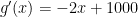
$g'(x) = -2x+1000$ will go to $-\infty$ as x approaches $\infty$ . $g'(x) \neq 0$ for any infinitely large x value since it just continues to go to $- \infty$ .

So we know that this limit meets all 3 requirements needed to apply L’Hospital’s Rule.

Now we know we can apply L’Hospital’s Rule

Taking the derivative of the top and bottom of the fraction individually tells us that:

$$\lim_{x \to \infty} \frac{e^x}{-x^2+1000x} = \lim_{x \to \infty} \frac{e^x}{-2x+1000}$$

Now we can evaluate this new limit instead. But if we do this, we will notice that we will still end up in the same situation that we had before.

$$\lim_{x \to \infty} \frac{e^x}{-2x+1000} \rightarrow \frac{\infty}{- \infty}$$

But what if it didn’t really help make the limit easier?

Which puts us in a perfect situation to consider using L’Hospital’s Rule to evaluate this new limit as well. By the same logic as before, we can confirm that the first two conditions are met as well as x gets infinitely large. Since all 3 required conditions are met we can go ahead and apply L’Hospital’s Rule a second time.

$$\lim_{x \to \infty} \frac{e^x}{-2x+1000} = \lim_{x \to \infty} \frac{e^x}{-2}$$

Now we can simply use the basic limit properties to evaluate this last limit.

Now we have a much easier limit

$$\lim_{x \to \infty} \frac{e^x}{-2} = \ – \frac{1}{2} \lim_{x \to \infty} e^x = \ – \infty$$

So therefore,

$$\lim_{x \to \infty} \frac{e^x}{-x^2+1000x} = \ – \infty$$

A quick note on applying L’Hospital’s Rule twice

This is an interesting problem because it shows that you can apply L’Hospital’s Rule multiple times on the same problem. You just need to make sure that each time you apply it, the resulting limit still meets all 3 required conditions before applying it to the new limit. There is no limit to the number of times you can continue applying L’Hospital’s Rule over and over in the same problem as long as you are making sure that the limit you are applying it to meets all 3 conditions every time you apply it.

Example 2

Evaluate the following limit using L’Hospital’s Rule or explain why L’Hospital’s Rule cannot be used to evaluate this limit.

$$\lim_{x \to 3} \frac{x-3}{27-x^3}$$

Again, if we think about what value the top and bottom of this fraction will go towards as x approaches 3, we would see that

$$\lim_{x \to 3} \frac{x-3}{27-x^3} \rightarrow \frac{0}{0}$$

Since we get another indeterminate form, which is $\frac{0}{0}$, we should consider using L’Hospital’s Rule to make this limit easier to evaluate.

So L’Hospital’s Rule might help…

First, we need to make sure that the other two conditions are met as well.

We can check that $g'(x) = -3x^2$ doesn’t equal zero anywhere near $x=3$ . This is because $g'(x) = -3x^2$ is continuous everywhere and the only place where $g'(x)=-3x^2=0$ is when $x=0$ . As a result of these two things, we can pick some interval around $x=3$ that doesn’t include $x=0$ to satisfy condition #2.

Also, both f(x) and g(x) are polynomials and are therefore differentiable everywhere. So we know they will both be differentiable on any interval around $x=3$ .

Now we know we can apply L’Hospital’s Rule

Doing so by taking the derivative of the top and bottom of our fraction separately tells us that

$$\lim_{x \to 3} \frac{x-3}{27-x^3} = \lim_{x \to 3} \frac{1}{-3x^2}$$

And doing this gives us an easier limit to deal with. Now we can simply apply the limit properties to evaluate. Applying the limit properties tells us that:

$$\lim_{x \to 3} \frac{1}{-3x^2} = \frac{1}{-3 \Big( \lim_{x \to 3}x \Big) ^2}= \frac{1}{-3(3)^2} = \ – \frac{1}{27}$$

So therefore we know that:

$$\lim_{x \to 3} \frac{x-3}{27-x^3} = \ – \frac{1}{27}$$

Example 3

Evaluate the following limit using L’Hospital’s Rule or explain why L’Hospital’s Rule cannot be used to evaluate this limit.

$$\lim_{x \to 0} \frac{|x|}{x^5+2x}$$

If we think about what value the numerator and denominator of this fraction will approach as x approaches 0 from both sides, we would see:

$$\lim_{x \to 0} \frac{|x|}{x^5+2x} \rightarrow \frac{0}{0}$$

Since we get an indeterminate form, which is $\frac{0}{0}$, we should consider using L’Hospital’s Rule to make this limit easier to evaluate.

So L’Hospital’s Rule might help…

First, we need to make sure that the other two conditions are met as well.

Upon checking condition #1 however, we run into a problem. Condition #1 requires that f(x) and g(x) are both differentiable on some interval containing $x=0$ , including $x=0$ .

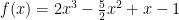
But $f(x) = |x|$ is not differentiable at $x=0$ . Therefore, we actually can’t apply L’Hospital’s Rule to evaluate this limit. I won’t go into the details here since we won’t be using L’Hospital’s Rule. But if you want to try evaluating this limit, I’d recommend considering both one-sided limits on their own and compare them to start. You can see a similar application here.

Example 4

$\mathbf{\lim\limits_{x \to \infty} \frac{ln(x)}{\sqrt{x}}}$ | Solution

Optimization Problems Part 2

In my last lesson, I introduced optimization problems and I discussed local extrema. You should check that out if you haven’t already. The next thing that I would like to discuss now is finding global maximums and minimums. The first step in finding a global maximum or minimum of a function is actually very similar to finding the local max and min values.

But once you know about the local maximums and minimums, how do you find the global extrema?

Finding the global extrema from the local extrema is really quite simple. And there really is only one way to find the global maximum and minimum values of a function. You just need to find a list of all possible x values where the global max or global min may occur. Then once you have created a list of all possibilities, you just plug them all into the original function.

Not the function’s derivative or the function’s second derivative. But the original function.

You will test for global extrema of f(x) using f(x), not f'(x) or f”(x). This is after you have your list of all possible locations where the global extrema could occur (which will require the use of f'(x)). But my point is that there wouldn’t be a first derivative test or a second derivative test with the global extrema like there was with finding local extrema.

So what does this look like in practice?

Let’s use an example. For example, let’s say that we are asked to find the global maximum and the global minimum of $f(x)=2x^3-\frac{5}{2}x^2+x-1$ on the domain $-4 \leq x \leq 5$ .

Notice we are being asked to find the global extrema on a specific domain. This is important because a lot of functions either go to infinity or to negative infinity as x either gets infinitely large, infinitely small, or approaches some specific value. So if we were asked to find the global maximum of a function that goes to infinity as x goes to infinity, we wouldn’t be able to do this. There would be no maximum since the function only continues to grow.

So we know we will be limited to a specific domain.

As I said before, finding global extrema starts out exactly like finding local extrema. The first thing we need to do is find the critical values of our function. To do this, we just need to find its derivative and set $f'(x)=0$ and solve for x.

$$f(x)=2x^3-\frac{5}{2}x^2+x-1$$ $$f'(x)=6x^2-5x+1$$ Then set $$6x^2-5x+1=0$$ and solve for x to find the critical values. To do this, we can factor the left side of the equation. $$(3x-1)(2x-1)=0$$ To solve this we can set each factor equal to zero individually. $$3x-1=0 \ \ \ \ and \ \ \ \ 2x-1=0$$ $$3x=1 \ \ \ \ and \ \ \ \ 2x=1$$ $$x=\frac{1}{3}, \ \frac{1}{2}$$

So now we know that this function has two critical values, $x= \frac{1}{3}$ and $x=\frac{1}{2}$ . Now this is where things get different with a global max/min problem versus finding the local max/min. We also need to consider the endpoints of our given domain as critical values!

This will always be the case when we are looking for a global maximum or minimum. The problem asked us to find the global extrema on the domain $-4 \leq x \leq 5$ . Therefore, we will also say that $x=-4$ and $x=5$ will be treated as critical values that we need to test.

So how to we test our critical values?

The first thing that I would like to do is list out all of the x values we will be testing in one place. Remember, the list of values we need to test came from two places:

Setting $f'(x)=0$ and solving for x.
Each of the endpoints of the domain on which we need to find the global maximums and minimums.

So in this case we’ll have four total x values that we need to test: $$x=-4, \ \frac{1}{3}, \ \frac{1}{2}, \ and \ 5$$ To test these points, all we need to do is plug each of the four points into f(x). Whichever on outputs the largest number will tell us the global maximum. Whichever outputs the smallest number will tell us the global minimum.

$$f(-4)= \ 2(-4)^3-\frac{5}{2}(-4)^2+(-4)-1 \ = -173$$ $$f \bigg( \frac{1}{3} \bigg) = \ 2 \bigg( \frac{1}{3} \bigg) ^3-\frac{5}{2} \bigg( \frac{1}{3} \bigg) ^2+ \bigg( \frac{1}{3} \bigg) -1 \ = -\frac{47}{54}$$ $$f \bigg( \frac{1}{2} \bigg) = \ 2 \bigg( \frac{1}{2} \bigg) ^3-\frac{5}{2} \bigg( \frac{1}{2} \bigg) ^2+ \bigg( \frac{1}{2} \bigg) -1 \ = -\frac{7}{8}$$ $$f(5)= \ 2(5)^3-\frac{5}{2}(5)^2+(5)-1 \ = \frac{383}{2}$$

So we can see that the smallest of these four numbers is -173 and the largest of them is $\frac{383}{2}$ . Therefore, the global maximum of f(x) on $-4 \leq x \leq 5$ is $\frac{383}{2}$ which occurs when $x=5$ . And the global minimum of f(x) on $-4 \leq x \leq 5$ is -173 which occurs when $x=-4$ .

We can even graph our function using Desmos along with the critical points to make sure our answer makes sense. You can click on the link in the last sentence to see a larger version of the graph.

global extrema maximum minimum — $f(x)=2x^3-\frac{5}{2}x^2+x-1$ on the domain $-4 \leq x \leq 5$

$f(x)=2x^3-\frac{5}{2}x^2+x-1$ on the domain $-4 \leq x \leq 5$

Extra practice

If you’d like some extra practice finding global maximums and minimums, here are a few examples you can work through on your own. A couple of these examples will require the use of the product rule and quotient rule.

For each of the following, find the global maximum and minimum of the given function on the given domain or explain why one doesn’t exist.

$$f(x)= 2x^4 + 5x^2 – 12x \ \ \textrm{on the domain} -1 \leq x \leq 2$$ $$g(x)= xe^x +6x^3-12 \ \ \textrm{on the domain} -3 \leq x \leq 0$$ $$h(x)= \frac{x^4-3x^2+1}{x+1} \ \ \textrm{on the domain} -2 \leq x \leq \frac{3}{2} $$ $$j(x)= \frac{x^4-3x^2+1}{x+1} \ \ \textrm{on the domain} -\frac{9}{10} \leq x \leq \frac{3}{2}$$

Hopefully all of this helps with global maximums and minimums, but as always I’d love to hear your questions if you have any. If you find that you get stuck as you’re working through some of these extra practice problems just let me know. Just email me at jakesmathlessons@gmail.com and I’ll see if I can help provide a bit more clarification. You can also use the form below to subscribe to my email list and I will send you my bonus FREE calculus 1 study guide to help you survive calculus! Just put in your name and email address and I’ll be sure to let you know when I post new content! Feel free to go check out my other lessons and solutions about derivatives as well.

Optimization Problems

Optimization problems are another common application of the derivative. Usually in these problems you are given some function or described some situation and are then asked to find different maximums and minimums. There are a few different things that are commonly asked that you optimize, so I’d like to go over the different categories with you.

Local maximums and minimums

The most common thing that comes up in optimization problems is finding the local maximums and minimums. The best way to do this is using the derivative of the function you are trying to optimize. Taking the function’s derivative will tell you everything you need to know.

In order to find the list of all x values where the local extrema may occur, you just need to take the function’s derivative, set it equal to zero, and solve for x. In other words, you can find the x values that will give you local max and min values by setting up the equation $$f'(x)=0$$ and solving it for x. Keep in mind, this equation often has multiple solutions, so make sure you include all possible solutions.

Doing this will give you a list of x values where all possible local maximums and minimums occur. These are called critical numbers.

Once you have your list of critical points, you will often need to figure out which ones are maximums and minimums. There are two tests you can conduct to figure which one they are.

First derivative test

This is usually the method I like to use. As you might guess, the first derivative test only requires the use of the first derivative. I usually use this test because we already had to find the first derivative to get our list of critical values.

The first thing I would suggest doing before beginning your test is drawing out a number line and putting your critical values on it. Let’s just say for example that we had some function f(x), took its derivative, and found that the critical values are $x=-1, \ 2, \ 6$ . Our number line might look something like this.

That’s all you need on your number line at this point. Don’t label any extra x values besides your critical values. It will only make things more confusing later.

Now all we need to do is plug x values into f’ that are around these critical values to figure out where f is increasing and decreasing. So we will need to plug in some number that is in each of the following 4 intervals. $$x<-1,$$ $$-1 < x < 2,$$ $$2 < x < 6,$$ $$x>6.$$ So all we need to do is just plug in some number in each segment of our labeled number line.

It doesn’t matter which number you plug in from each of those intervals, so you can pick whichever numbers seem easiest to plug into f’. Let’s say we will plug $x=-2, \ 0, \ 4, \ 7$ into f’. We want to plug them into f’ because we are trying to figure out information about the slope of f. This will tell us where it’s increasing and decreasing. Let’s imagine we plug these four x values into f’ and find that $$f'(-2)=-4, \ \ \ f'(0)=6, \ \ \ f'(4)=2, \ \ \ f'(7)=-7.$$

We only really care if these values are positive or negative. If f’ is positive at a certain x value, we know f must have a positive slope. And if f’ is negative at a certain x value, we know f must have a negative slope.

Since f'(-2) is negative, f must have a negative slope at $x=-2$ . And f must also have a negative slope for all $x<-1$ since that is the interval from our number line that $x=-2$ falls within. So we should label this interval with a negative slope, like this:

critical values number line labeled with slope

Then we want to do the same thing for the interval of $-1 \leq x \leq 2$ . We found out that $f'(0)=6$ , which is a positive number. Therefore, f must have a positive slope for all $-1 \leq x \leq 2$ . So we can label our number line accordingly.

Then we want to do the same thing with the other two intervals. This would give us something like this for our number line:

Now we just need to use this number line to determine which critical values are maximums and which are minimums. There are really only 3 main cases you need to think about for each critical value.

If f is increasing to the left and decreasing to the right, that critical point will be a local maximum. This will cause this little section of the graph to look like a frowny face. Therefore, the critical point will higher than the graph right around it.
If f is decreasing to the left and increasing to the right, that critical point will be a local minimum. This will cause this little section of the graph to look like a smiley face. Therefore, the critical point will lower than the graph right around it.
If f is decreasing to the left and the right or if it’s increasing to the left and the right, that critical point will NOT be a local maximum or a local minimum.

So let’s look at each of our three critical values on the number line above and see which category they all fall into.

For $x=-1$ , you can see that f is decreasing on the left side and increasing on the right side. Therefore, the section of the f(x) right around $x=-1$ looks like a smiley face and would be a local minimum.
For $x=2$ , you can see that f is increasing on the left side and increasing on the right side. Therefore, the critical value $x=2$ would not be a local maximum or a local minimum. We would need f(x) to change direction at $x=2$ for it to be a maximum or minimum, but that doesn’t happen here.
For $x=6$ , you can see that f is increasing on the left side and decreasing on the right side. Therefore, the section of the f(x) right around $x=6$ looks like a frowny face and would be a local maximum.

Second derivative test

The other way you can test to see if each critical value is a local maximum or a local minimum is with the second derivative test. You do not need to use both methods if you are only trying to find local extrema because they will give you the same conclusions. Just pick which test you like more. This method will require us to find the second derivative of our function, or f”(x). We can find this simply by finding the derivative of f'(x), which we already found.

Just like with the first derivative test, it helps to draw everything out on a number line. Start with just drawing a number line that only contains the critical values which we found a while ago.

Now we need to plug each of our critical values into our second derivative, or f”(x). One important difference is that we had to plug numbers around our critical values with the first derivative test. But with the second derivative test, we will actually plug in the critical values instead of numbers around them.

Since we need to plug each critical value into our second derivative, this means we will plug $x=-1, \ \ 2, \ \ 6$ into f”(x). When we do that, let’s imagine we find that $$f”(-1) = 2, \ \ f”(2) = 0, \ \ f”(6) = -9.$$

Just like before, it doesn’t really matter what the exact values are that we just found. All that matters is whether they are positive, negative, or zero. If f” is positive at a certain point, then f would be concave up at that point. And if f” is negative at a point, then f is concave down at that point. If f” is zero, then f isn’t concave up or concave down at that point.

Since f”(-1) is positive (we just found that it’s 2), we know that f is concave up when $x=-1$ . That just means that it’s curved upward, like a smiley face. So we can indicate this on our number line to keep track of what we have so far.

critical values number line labeled with concavity

Since f”(2) is zero, we know that f is not concave up or down when $x=2$ . This tells us that $x=2$ is the point where f switches from being concave up to concave down, or vise versa. Since f doesn’t have concavity (curvature) here, we will show this as a flat line on our number line.

And lastly, since f”(6) is negative (we just found that it’s -9), we know that f is concave down when $x=6$ . That just means that it’s curved downward, like a frowny face. Therefore, we might get something like this.

So now we just need to figure out what all this means when it comes to the second derivative test. Again, there are three cases we want to look for.

If f(x) is concave up, or f”(x) is positive, for some critical value x, then this critical value represents a local minimum.
If f(x) is concave down, or f”(x) is negative, for some critical value x, then this critical value represents a local maximum.
If f(x) isn’t concave up or down, or f”(x) is zero, for some critical value x, then this critical value could be a local minimum or local maximum or neither.

So let’s compare these to our critical values to see if they are each local maximums or minimums.

For $x=-1$ , you can see that f is concave up. Therefore, the section of the f(x) right around $x=-1$ looks like a smiley face and would be a local minimum.
For $x=2$ , you can see that f is not concave up or concave down. In this case we don’t know from the second derivative test if this critical value would be a local maximum or a local minimum.
For $x=6$ , you can see that f is concave down. Therefore, the section of the f(x) right around $x=6$ looks like a frowny face and would be a local maximum.

Notice that these are the exact same results we found from the first derivative test, aside from the undetermined critical value. I know we didn’t actually have a function for f(x) to work through, but you would find the same thing if you did actually go through these processes with some function. To find which critical values are local maximums, local minimums, or neither, you only need to do one of these two tests.

Extra practice

Find the critical values for the following functions and determine whether each one is a local minimum, local maximum, or neither. A couple of these examples will require the use of the product rule and the quotient rule, so check those out if you need a refresher.

$$f(x)= 2x^4 + 5x^2 – 12x$$ $$g(x)= xe^x +6x^3-12$$ $$h(x)= \frac{x^4-3x^2+1}{x+1}$$

Hopefully all of this helps you gain a bit of a better understanding of local extrema, but as always I’d love to hear your questions if you have any. Go check out part 2 of my coverage on optimization problems where I go over global maximums and minimums.

How to find the equation of a tangent line

One common application of the derivative is to find the equation of a tangent line to a function. Usually when you’re doing a problem like this, you will be given a function whose tangent line you need to find. And you will also be given a point or an x value where the line needs to be tangent to the given function.

Using these two pieces of information, you need to create an equation for a line that satisfies the required conditions. This process is very closely related to linear approximation (or linearization) and differentials.

When coming up with the equation of the line, there are a couple different approached you could take. You should decide which one to use based on your own personal preference. The only difference between the different approaches is which template for an equation of a line you prefer to use. Remember, there are two main forms that a line will take: $$y=mx+b$$ $$y=m(x-x_0)+y_0$$ Another thing to keep in mind is that the first form is generally easier when we are given the y-intercept of the line. The second form above is usually easier when we are given any other point that isn’t the y-intercept.

In both of these forms, x and y are variables and m is the slope of the line. In the first equation, b is the y-intercept. And in the second equation, $x_0$ and $y_0$ are the x and y coordinates of some point that lies on the line. This could be any point that lies on the line.

It is also important to notice that a line would be tangent to a function at a specific point if and only if the following two conditions are met.

The function and its tangent line need to go through the same point
and they both need to share the same slope at that shared point.

But how does the derivative apply?

You should always keep in mind that a derivative tells you about the slope of a function. So if we take a function’s derivative, then look at it at a certain point, we have some information about the slope of the function at that point. Since a tangent line has to have the same slope as the function it’s tangent to at the specific point, we will use the derivative to find m.

So let’s jump into a couple examples and I’ll show you how to do something like this.

Example 1

Find the equation of the tangent line to the function $\mathbf{y=x^3+4x-6}$ at the point (2, 10).

In order to find this tangent line, let’s consider the two conditions that need to be met for our line to be a tangent line at the specified point.

The tangent line and the given function need to go through the same point. Since the problem told us to find the tangent line at the point $(2, \ 10)$ , we know this will be the point that our line has to go through.
The tangent line and the function need to have the same slope at the point $(2, \ 10)$ . In order to find this slope we will need to use the derivative. Let’s start with this.

Finding the slope of the tangent line

Remember that the derivative of a function tells you about its slope. So to find the slope of the given function $y=x^3+4x-6$ we will need to take its derivative. This will just require the use of the power rule. $$y’=3x^2+4$$

But how can we use this to find the slope of the tangent line when it has variables in it?

This is where the specific point we need to consider comes into play. We know that the tangent line and the function need to have the same slope at the point $(2, \ 10)$ . Therefore, they need to have the same slope when $x=2$ . In order to find the slope of the given function y at $x=2$ , all we need to do is plug 2 into the derivative of y.

Therefore, the slope of our line would simply be $$y'(2)=3(2)^2+4=16.$$ And because of this we also know the slope of our tangent line will be $$m=16.$$ So we know this will guarantee that our tangent line has the right slope, now we just need to make sure it goes through the right point.

Making sure the tangent line contains the given point

Since we do know a point that has to lie on our line, but don’t know the y-intercept of the line, it would be easier to use the following form for our tangent line equation. $$y=m(x-x_0)+y_0$$

And since we already know $m=16$ , let’s go ahead and plug that into our equation. $$y=16(x-x_0)+y_0$$

Now to finish our tangent line equation, we just need the x and y coordinates of a point that lies on this line. Then we can simply plug them in for $x_0$ and $y_0$ . Well, we were given this information! We were told that the line we come up with needs to be tangent at the point $(2, \ 10)$ . Therefore, our tangent line needs to go through that point. This tells us our tangent line equation must be $$y=16(x-2)+10$$ $$y=16x-32+10$$ $$y=16x-22$$

And that’s it! We know that the line $y=16x-22$ will go through the point $(2, 10)$ on our original function. And we know that it will also have the same slope as the function at that point.

We can even use Desmos to check this and see what our function and tangent line look like together.

tangent line to a function — $y=x^3+4x-6$ and $y=16x-22$

Example 2

Find the equation of the line that is tangent to the function $f(x) = xe^x$ when $x=0$ .

To start a problem like this I suggest thinking about the two conditions we need to meet.

The tangent line and the given function need to intersect at $\mathbf{x=0}$ . This time we weren’t given the y coordinate of this point so we will need to figure that out.
Then we need to make sure that our tangent line has the same slope as f(x) when $\mathbf{x=0}$ .

Finding the slope of the tangent line

I personally think that it’s a little easier to find the slope of the tangent line first, but you can start with making sure the other condition is met if you prefer.

When you’re asked to find something to do with slope, your first thought should be to use the derivative. The derivative of a function tells you about it’s slope. Since we need the slope of f(x), we’ll need its derivative.

Looking at our function $f(x)=xe^x$ you can see that it is the product of two simpler functions. To find it’s derivative we will need to use the product rule. I’m not going to show every step of this, but if you aren’t 100% sure how to find this derivative you should click the link in the last sentence. $$f'(x) = e^x + xe^x$$ $$f'(x) = e^x \big(1+x \big)$$

Now consider the fact that we need our tangent line to have the same slope as f(x) when $x=0$ . To find the slope of f(x) at $x=0$ we just need to plug in 0 for x into the equation we found for f'(x). $$f'(0) = e^{(0)} \big( 1 + (0) \big)$$ $$f'(0) = 1(1)=1$$

So we know that the slope of our tangent line needs to be 1.

Making sure the tangent line contains the required point

Now we just need to make sure that our tangent line shares the same point as the function when $x=0$ . In order to do this, we need to find the y value of the function when $x=0$ . This would be the same as finding f(0). $$f(0) = (0)e^{(0)} = 0$$

Since this is the y value when $x=0$ , we can also say that this is the y-intercept. We know the y intercept of our tangent line is 0. Since we figured out the y-intercept, it would be easiest to use the $y=mx+b$ form of the line for the tangent line equation.

We already found that the slope will be 1 and that the y-intercept will need to be 0, so we can plug these values in for m and b. Doing this tells us that the equation of our tangent line is $$y=(1)x+(0)$$ $$y=x.$$

Again, we can see what this looks like and check our work by graphing these two functions with Desmos.

tangent lines example 2 — $y=xe^x$ and $y=x$

Finding the Tangent Line Equation with Implicit Differentiation

Depending on the curve whose tangent line equation you are looking for, you may need to apply implicit differentiation to find the slope.

Example 3

Find the equation of the line that is tangent to the curve $\mathbf{y^3+xy-x^2=9}$ at the point (1, 2).

First we need to apply implicit differentiation to find the slope of our tangent line.

$$\frac{d}{dx} \big[ y^3 + xy – x^2 \big] = \frac{d}{dx} [9]$$ $$3y^2 \frac{dy}{dx} + 1\cdot y + x \cdot \frac{dy}{dx} – 2x = 0$$ $$3y^2 \frac{dy}{dx} + x \frac{dy}{dx} = -y + 2x$$ $$\frac{dy}{dx} \big[ 3y^2 + x \big] = -y + 2x$$ $$\frac{dy}{dx} = \frac{-y+2x}{3y^2+x}$$

Now we can plug in the given point (1, 2) into our equation for $\mathbf{\frac{dy}{dx}}$ to find the slope of the tangent line.

$$m=\frac{-(2)+2(1)}{3(2)^2+(1)}=\frac{0}{13}=0$$

With this slope, we can go back to the point slope form of a line. Since we know the slope and a point that lies on this line, we can plug that information into the general point slope form for a line. This will leave us with the equation for a tangent line at the given point.

$$y=m(x-x_0)+y_0$$ $$y=0(x-1)+2$$ $$y=2$$

So the constant function $\mathbf{y=2}$ is tangent to the curve $\mathbf{y^3+xy-x^2=9}$ at the point (1, 2).

Example 4

Find the equation of the line that is tangent to the curve $\mathbf{16x^2 + y^2 = xy + 4}$ at the point (0, 2).

Again, we will start by applying implicit differentiation to find the slope of the tangent line.

$$\frac{d}{dx} \big[ 16x^2 + y^2 \big] = \frac{d}{dx} [xy + 4]$$ $$32x + 2y \frac{dy}{dx} = 1\cdot y + x \cdot \frac{dy}{dx}$$ $$2y \frac{dy}{dx} – x \frac{dy}{dx}= -32x + y$$ $$\frac{dy}{dx} \big[ 2y-x \big] = -32x+y$$ $$\frac{dy}{dx} = \frac{-32x+y}{2y-x}$$

Now we can plug in the given point (0, 2) into our equation for $\mathbf{\frac{dy}{dx}}$ to find the slope of the tangent line.

$$m = \frac{-32(0)+(2)}{2(2)-(0)}$$ $$m=\frac{2}{4}$$ $$m=\frac{1}{2}$$

$$y=m(x-x_0)+y_0$$ $$y=\frac{1}{2}(x-0)+2$$ $$y=\frac{1}{2}x+2$$

Tangent Line Equation Without Derivatives

There are some cases where you can find the slope of a tangent line without having to take a derivative. This is not super common because it does require being able to take advantage of additional information. Usually you will be able to do this if you know some geometrical fact about the curve whose tangent line equation you are looking for.

The most common example of this is finding the a line that is tangent to a circle.

Example 5

Find the equation of the line that is tangent to the circle $\mathbf{(x-2)^2+(y+1)^2=25}$ at the point (5, 3).

We already are given a point that we know needs to lie on our tangent line. This tells us that if we can find the slope of the tangent line, we would just be able to plug it all into the point slope form for a linear function and we would have a tangent line. So we just need to find the slope of the tangent line.

In order to find this slope we can take advantage of a geometrical fact about circles: a line connecting the center of a circle to its edge will be perpendicular to a line that is tangent to the circle at that edge point. Below you can see what this looks like on a graph of this circle, or at least a portion of it.

Graph of a circle and its tangent line — $\mathbf{(x-2)^2+(y+1)^2=25}$ and the tangent line at *(5, 3)*

$\mathbf{(x-2)^2+(y+1)^2=25}$ and the tangent line at *(5, 3)*

Therefore, if we know the slope of a line connecting the center of our circle to the point (5, 3) we can use this to find the slope of our tangent line. Based on the general form of a circle, we know that $\mathbf{(x-2)^2+(y+1)^2=25}$ is the equation for a circle that is centered at (2, -1) and has a radius of 5. So we need to find the slope of a line connecting the points (5, 3) and (2, -1). We can do this using the formula for the slope of a line between two points.

$$slope = \frac{y_2 – y_1}{x_2 – x_1}$$ $$slope = \frac{3 – (-1)}{5 – 2}$$ $$slope = \frac{4}{3}$$

Now we can simply take the negative reciprocal of $\mathbf{\frac{4}{3}}$ to find the slope of our tangent line. So we know the slope of our tangent line will be $\mathbf{- \frac{3}{4}}$ .

Knowing that the slope of our tangent line will be $\mathbf{- \frac{3}{4}}$ and that it will go through the point (5, 3), we can put this into the point slope form of a line to find the equation of our tangent line.

$$y=m(x-x_0)+y_0$$ $$y= \ – \frac{3}{4}(x-5)+3$$ $$y= \ – \frac{3}{4}x + \frac{15}{4}+3$$ $$y= \ – \frac{3}{4}x + \frac{15}{4}+ \frac{12}{4}$$ $$y= \ – \frac{3}{4}x + \frac{27}{4}$$

Hopefully all of this helps you gain a bit of a better understanding of finding tangent lines, but as always I’d love to hear your questions if you have any. Just email me at jakesmathlessons@gmail.com and I’ll see if I can help provide a bit more clarification. You can also use the form below to subscribe to my email list and I’ll send you my FREE bonus study guide to help you survive calculus! Just put in your name and email address and I’ll be sure to let you know when I post new content! Feel free to go check out my other lessons and solutions about derivatives as well.

Cylinder/Shell Method – Rotate around a horizontal line

Before reading through this problem, I’d recommend checking out my lesson on finding volumes of rotation using the cylinder shell method. I’m not going to go into quite as much detail here as I did in that lesson. It might help you make more sense of what’s going on if your start there.

Other than that there isn’t much else to add so let’s jump into an example!

Example 1

Find the area of the solid created by rotating the area bounded between $y= (x-1)^3-3$ , $y=-x-2$ , and $y=-2$ about the line $y=-1$ .

Just as before I’ll use the same 4 step process as in the cylinder method lesson.

1. Graph the 2-D functions

As I always say, I suggest starting any problem possible by drawing what is being described to you. Go ahead and start with graphing all of the functions described in the problem. I’ll do this using Desmos. You should end up with something like the graph below. I also went ahead and shaded the bounded region gray to make it a little easier to see (this was not done in Desmos).

$y= (x-1)^3-3$ , $y=-x-2$ , $y=-2$ , and $y=-1$

$y= (x-1)^3-3$ , $y=-x-2$ , $y=-2$ , and $y=-1$

2. Rotate the 2-D area around the given axis

Again, we want to visualize what the question is asking us to find. We will need to take the shaded region in the above graph and rotate it around the line $y=-1$ . Doing this would create a 3-D figure whose volume we’ll need to find. But first let’s draw it.

To do this, imagine the 2-D gray region coming off the paper or screen and rotating around the axis of rotation. Doing this would give us something like the figure below.

Figure resulting from rotating the area around a horizontal. — Result of rotating the region about the line $y=-1$ .

Result of rotating the region about the line $y=-1$ .

3. Setting up the integral

I’m not going to go into as much detail to explain where this integral comes from as I did in the cylinder method lesson, but if the following integral confuses you I’d recommend checking that lesson out by clicking on the above link.

Long story short, we want to imagine our 3-D figure is made up of several infinitely thin cylindrical shells. Adding up the volume of all of these shells would result in an integral like this: $$\int 2 \pi r h \ dr.$$

In order to help with coming up with each of these pieces, we need to relate them back to our figure and the functions that created it. In order to visualize this, let’s draw our figure with one of these infinitely thin shells that make up the entire figure. We can consider this one shell and how to represent these dimensions in terms of the given functions.

You can see one of these cylindrical shells represented in the drawing below with a labeled version of the cylinder draw in the upper-right hand corner.

3-D figure with a cylindrical shell — 3-D figure with a sample cylindrical shell shown in green.

As with all cylinder shell method problems, we need to imagine integrating from the center of the cylinder out to the outer edge. Since our cylinder is laying horizontally, moving from its center to its edge moves up and down. This means we are moving in the y direction. Therefore, we need to integrate in the y direction and represent our integral only in terms of y (we shouldn’t have any x‘s).

So let’s think about each of the three pieces that make up our integral one at a time.

Finding r

The radius of this cylinder would simply be the distance between the center of the cylinder and the edge. You can see in the smaller version of the cylinder drawn off to the side that the radius is represented by the red line measuring between the points labeled $(x_2, \ -1)$ and $(x_2, \ y)$ .

Since these two points have the same x value, we can find the distance between them by simply finding the distance between their y values. To do this we just need to take the larger value and subtract the smaller one from it. $$r=-1-y$$

Finding h

The height of a cylinder will always be measured as the distance between the two flat, parallel faces. Usually they would be the top and bottom, but since our cylinder is sideways, we need the distance between the left side and right side.

Looking at the smaller cylindrical shell off to the side in the drawing above, you can see the height of this cylinder is represented by the red line measuring the distance between the points $(x_1, \ y)$ and $(x_2, \ y)$ .

Similar to what we did before, these two points have the same y value. As a result, the distance between them would be the same as the distance between their x values. So we just need to take the larger x value and subtract away the smaller one. $$h=x_2-x_1$$

But remember earlier I said we need everything just in terms of y?

So we need to think about how we can rewrite $x_1$ and $x_2$ in terms of y.

Finding $\mathbf{x_1}$

We know that $x_1$ lies on the function $y=-x-2$ so we know that the relationship between $x_1$ and y can be described in the same way $$y=-x_1-2.$$ If we rearrange this to solve for $x_1$ instead of y, we can use this to replace the $\mathbf{x_1}$ in our equation for h. $$y=-x_1-2$$ $$y+x_1=-2$$ $$x_1=-y-2$$

We can use this to rewrite h but replace the $x_1$ with $(-y-2)$ since we know they are equal. $$h= \ x_2- (-y-2)$$ Now we need to do the same thing with $x_2$ .

Finding $\mathbf{x_2}$

We are going to apply the same idea here as in the previous section. We know that $x_2$ lies on the function $y= (x-1)^3-3$ . Therefore, we can describe the relationship between $x_2$ and y as $$y= (x_2-1)^3-3.$$ Now we can solve this equation for $x_2$ and plug this into our equation for h. $$y \ = \ (x_2-1)^3-3$$ $$y+3 \ = \ (x_2-1)^3$$ $$\sqrt[3] {y+3} \ = \ x_2-1$$ $$\sqrt[3] {y+3} +1 \ = \ x_2$$ Now going back to our equation for h, this tells us $$h \ = \ \sqrt[3] {y+3} +1 – (-y-2).$$ And to simplify a bit: $$h \ = \ \sqrt[3] {y+3} +1 + y+2$$ $$h \ = \ \sqrt[3] {y+3} + y+3.$$ Now that we have h and r, we just need to find dr.

Finding dr

This is actually the simplest part to find. The dr represents the change in the cylinder’s radius as we go from each shell to the next. Since we move in the same direction of the radius as we integrate to find our volume, the change in r should be the same as the change in y between each step. Therefore, we can say that $$dr=dy.$$

Putting it all back into an integral

We already figured out that the volume of our figure can be found by using the integral $$\int 2 \pi rh \ dr.$$ And we just found these three pieces to be $$r=-1-y$$ $$h \ = \ \sqrt[3] {y+3} + y+3$$ $$dr=dy.$$ So we can just plug them into our integral. $$ \int 2 \pi \ ( -1-y ) \ \Big( \sqrt[3] {y+3} + y+3 \Big) \ dy$$

Now we need one last piece. We need to add bounds on the integrals.

Since we are integrating with respect to y, the bounds of our integrals need to be the range of y values that make up our original 2-D area. Looking back at our original graph, we can see that the original area bounded by the given functions spans over all of the y values between $y=-2$ and $y=-3$ . Therefore, we know that the volume of our figure will be $$V \ = \int_{-3}^{-2} 2 \pi \ ( -1-y ) \ \Big( \sqrt[3] {y+3} + y+3 \Big) \ dy.$$

4. Solve the integral

Now all we need to do is solve the integral we just found and that will leave us with our volume. This is actually a pretty complicated integral as is it, so let’s start with simplifying it a bit. We’ll do this by pulling out the constant, distributing out through the parenthesis, and combining like terms.

$$V \ = \int_{-3}^{-2} 2 \pi \ ( -1-y ) \ \Big( \sqrt[3] {y+3} + y+3 \Big) \ dy$$ $$V \ = \ 2 \pi \int_{-3}^{-2} \ – \big(y+3 \big)^{\frac{1}{3}} – y \ – 3 -y \big(y+3 \big)^{\frac{1}{3}} – y^2 – 3y \ \ dy$$ $$V \ = \ 2 \pi \int_{-3}^{-2} \ – \big(y+3 \big)^{\frac{1}{3}} -y \big(y+3 \big)^{\frac{1}{3}} – y^2 – 4y -3 \ \ dy$$

Now that we have it in a form that is simplest to integrate we can go ahead and integrate this function one term at a time. I’m not going to show every step of how to do this, but if you’d like to work it out on your own, I’d suggest using u-substitution on the $-(y+3)^{1/3}$ term and using integration by parts on the $-y(y+3)^{1/3}$ term.

$$V \ = \ 2 \pi \Bigg[ – \frac{3}{14} \big( y+3 \big)^{\frac{4}{3}}\big( 2y-1 \big) – \frac{1}{3}y^3 – 2y^2 – 3y \Bigg]_{-3}^{-2}$$

Again, I’m not going to show every step of this. Instead I used Wolfram Alpha from here, but if you evaluate this expression from $y=-3$ to $y=-2$ , you’ll see that $$V \ = \ 2 \pi \bigg(\frac{73}{42} \bigg)$$ $$V \ = \ \frac{73 \pi}{21}$$

Hopefully all of this helps you gain a bit of a better understanding of this method, but as always I’d love to hear your questions if you have any. Just email me at jakesmathlessons@gmail.com and I’ll see if I can help provide a bit more clarification. You can also use the form below to subscribe to my email list and I’ll send you my bonus FREE calc 1 study guide! Just put in your name and email address and I’ll be sure to let you know when I post new content! Feel free to go check out my other lessons and solutions about integrals as well.

x	$\mathbf{\frac{1}{x}}$
1	1
10	0.1
100	0.01
1,000	0.001
10,000	0.0001
100,000	0.00001
1,000,000	0.000001
10,000,000	0.0000001
100,000,000	0.00000001

x	$\mathbf{e^x}$
1	2.718
2	7.389
4	54.598
6	403.429
8	2,980.958
10	22,026.466
100	2.688 * $\mathbf{10^{43}}$